Upscaling and Inverse Modeling of Groundwater Flow and Mass ...

CHAPTER 5. JOINTLY MAPPING HYDRAULIC . . . 117
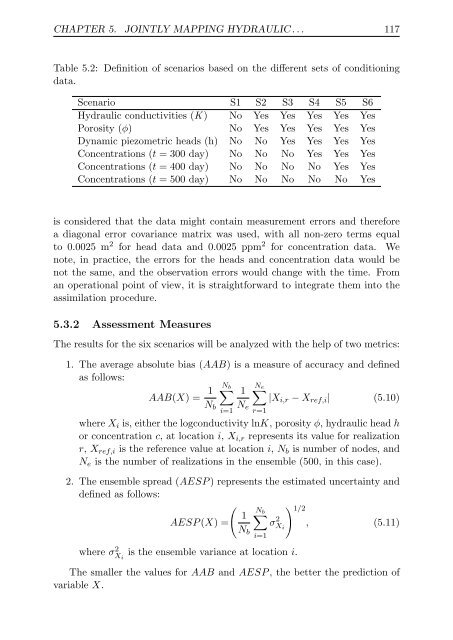
Table 5.2: Definition of scenarios based on the different sets of conditioning
data.
Scenario S1 S2 S3 S4 S5 S6
Hydraulic conductivities (K ) No Yes Yes Yes Yes Yes
Porosity (ϕ) No Yes Yes Yes Yes Yes
Dynamic piezometric heads (h) No No Yes Yes Yes Yes
Concentrations (t = 300 day) No No No Yes Yes Yes
Concentrations (t = 400 day) No No No No Yes Yes
Concentrations (t = 500 day) No No No No No Yes
is considered that the data might contain measurement errors and therefore
a diagonal error covariance matrix was used, with all non-zero terms equal
to 0.0025 m 2 for head data and 0.0025 ppm 2 for concentration data. We
note, in practice, the errors for the heads and concentration data would be
not the same, and the observation errors would change with the time. From
an operational point of view, it is straightforward to integrate them into the
assimilation procedure.
5.3.2 Assessment Measures
The results for the six scenarios will be analyzed with the help of two metrics:
1. The average absolute bias (AAB) is a measure of accuracy and defined
as follows:
AAB(X) = 1
Nb Ne ∑ 1 ∑
|Xi,r − Xref,i| (5.10)
Nb
Ne
i=1 r=1
where Xi is, either the logconductivity lnK, porosity ϕ, hydraulic head h
or concentration c, at location i, Xi,r represents its value for realization
r, Xref,i is the reference value at location i, Nb is number of nodes, and
Ne is the number of realizations in the ensemble (500, in this case).
2. The ensemble spread (AESP ) represents the estimated uncertainty and
defined as follows:
(
Nb
1 ∑
AESP (X) = σ 2 ) 1/2
Xi , (5.11)
where σ 2 Xi
Nb
i=1
is the ensemble variance at location i.
The smaller the values for AAB and AESP , the better the prediction of
variable X.