Upscaling and Inverse Modeling of Groundwater Flow and Mass ...

CHAPTER 5. JOINTLY MAPPING HYDRAULIC . . . 111
locations, and, in our case, is composed of 0 ′ s and 1 ′ s since we
assume that measurements are taken at block centers. Therefore,
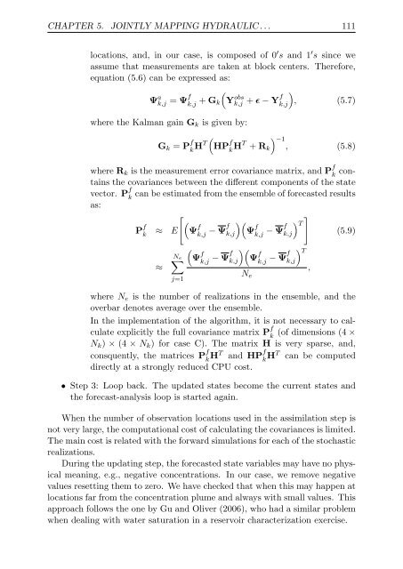
equation (5.6) can be expressed as:
Ψ a k,j
= Ψf
k,j + Gk
where the Kalman gain Gk is given by:
(
Y obs
k,j + ϵ − Yf
k,j
)
, (5.7)
Gk = P f
(
kHT HP f
kHT ) −1
+ Rk , (5.8)
where Rk is the measurement error covariance matrix, and P f
k con-
tains the covariances between the different components of the state
vector. P f
k can be estimated from the ensemble of forecasted results
as:
P f
[
(
k ≈ E Ψ f
)(
k,j − Ψfk,j
Ψ f
]
) T
k,j − Ψfk,j
(5.9)
≈
Ne ∑
j=1
(
Ψ f
)(
k,j − Ψfk,j
Ψ f
) T
k,j − Ψfk,j
where Ne is the number of realizations in the ensemble, and the
overbar denotes average over the ensemble.
In the implementation of the algorithm, it is not necessary to calculate
explicitly the full covariance matrix P f
k (of dimensions (4 ×
Nk) × (4 × Nk) for case C). The matrix H is very sparse, and,
consquently, the matrices P f
kHT and HP f
kHT can be computed
directly at a strongly reduced CPU cost.
• Step 3: Loop back. The updated states become the current states and
the forecast-analysis loop is started again.
When the number of observation locations used in the assimilation step is
not very large, the computational cost of calculating the covariances is limited.
The main cost is related with the forward simulations for each of the stochastic
realizations.
During the updating step, the forecasted state variables may have no physical
meaning, e.g., negative concentrations. In our case, we remove negative
values resetting them to zero. We have checked that when this may happen at
locations far from the concentration plume and always with small values. This
approach follows the one by Gu and Oliver (2006), who had a similar problem
when dealing with water saturation in a reservoir characterization exercise.
Ne
,