Upscaling and Inverse Modeling of Groundwater Flow and Mass ...

Recommendations

Info

152 CHAPTER 6. GROUNDWATER FLOW INVERSE MODELING . . . 240 North (A) Correct P rior: 1st Realization .0 .0 East 300 240 North (D) W rong P rior: 1st Realization .0 .0 East 300 3.0 2.0 1.0 .0 -1.0 -2.0 -3.0 3.0 2.0 1.0 .0 -1.0 -2.0 -3.0 Frequency Frequency 0.120 0.080 0.040 0.000 0.120 0.080 0.040 0.000 (B) Correct Prior -4.0 -2.0 0.0 2.0 4.0 (E) Wrong Prior value value Number of Data 8000 mean -0.51 std. dev. 1.56 coef. of var undefined maximum 3.44 upper quartile 0.67 median -1.16 lower quartile -1.51 minimum -3.39 Number of Data 8000 mean -0.54 std. dev. 1.47 coef. 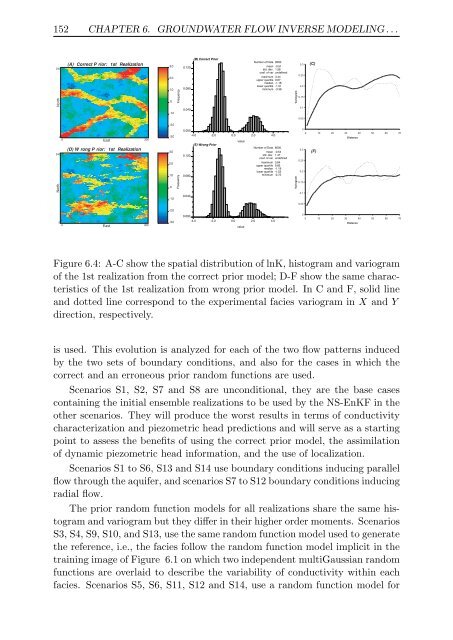of var undefined maximum 3.64 upper quartile 0.85 median -1.19 lower quartile -1.53 minimum -2.72 -4.0 -2.0 0.0 2.0 4.0 Variogram 0.3 0.25 0.2 0.15 0.1 0.05 (C) 0 0 10 20 30 40 50 60 70 0.3 0.25 0.2 0.15 0.1 0.05 Distance 0 0 10 20 30 40 50 60 70 Figure 6.4: A-C show the spatial distribution of lnK, histogram and variogram of the 1st realization from the correct prior model; D-F show the same characteristics of the 1st realization from wrong prior model. In C and F, solid line and dotted line correspond to the experimental facies variogram in X and Y direction, respectively. is used. This evolution is analyzed for each of the two flow patterns induced by the two sets of boundary conditions, and also for the cases in which the correct and an erroneous prior random functions are used. Scenarios S1, S2, S7 and S8 are unconditional, they are the base cases containing the initial ensemble realizations to be used by the NS-EnKF in the other scenarios. They will produce the worst results in terms of conductivity characterization and piezometric head predictions and will serve as a starting point to assess the benefits of using the correct prior model, the assimilation of dynamic piezometric head information, and the use of localization. Scenarios S1 to S6, S13 and S14 use boundary conditions inducing parallel flow through the aquifer, and scenarios S7 to S12 boundary conditions inducing radial flow. The prior random function models for all realizations share the same histogram and variogram but they differ in their higher order moments. Scenarios S3, S4, S9, S10, and S13, use the same random function model used to generate the reference, i.e., the facies follow the random function model implicit in the training image of Figure 6.1 on which two independent multiGaussian random functions are overlaid to describe the variability of conductivity within each facies. Scenarios S5, S6, S11, S12 and S14, use a random function model for Variogram (F) Distance
CHAPTER 6. GROUNDWATER FLOW INVERSE MODELING . . . 153 the facies based on the indicator variogram computed on the training image on which the same independent multiGaussian random functions of the reference field are overlaid. For the first set of scenarios the multiple point code SNESIM Strebelle (2002) is used to generate the facies realizations, whereas the indicator simulation code ISIM3D (Gómez-Hernández and Srivastava, 1990) is used for the second set. The parameters defining the two multiGaussian random functions are given in Table 6.1. Figure 6.4 shows the first realization for the correct and the incorrect model, their histograms and their variograms. While both realizations follow the same histogram and variograms, the variogrambased sequential indicator simulation cannot generate the curvilinear patters for the sand facies observed in the training image, which are well reproduced in the multipoint sequential simulation. For the scenario S3, S5, S9, S11, S13 and S14 head data are assimilated without using localization whereas for the scenarios S4, S6, S10 and S12 localization is employed. The EnKF tends to filter inbreeding if the ensemble size is small, and the heterogeneity is large (Hendricks Franssen and Kinzelbach, 2009). It is therefore expected that the NS-EnKF applied to a complex geological environment will suffer this problem, too. To analyze this aspect, a fifth-order distancedependent localization function (Hamill et al., 2001) is used to reduce the sampling errors in the computation of the ensemble covariances. Considering previous works (Chen and Oliver, 2010), the size of the domain, the separation between piezometers, and the distance between wells for the boundary conditions inducing radial flow, the localization function is set to zero at a distance of 80 m, implying that for distances larger than that, the sampled non-stationary covariances used to compute the Kalman gain are zero. More specifically, the distance function that is used for both ρ ˆ X ˆ Y and ρ ˆ Y ˆ Y in Equation (6.5) is: ⎧ ⎪⎨ − Ω(d) = ⎪⎩ 1 d 4 ( 1 d 12 ( 40 )5 + 1 d 2 ( 40 )4 + 5 d 8 ( 40 )3 − 5 d 3 ( 40 )2 + 1, 0 ≤ d ≤ 40; 40 )5 − 1 d 2 ( 40 )4 + 5 d 8 ( 40 )3 + 5 d 3 ( 40 )2 − 5( d 2 d 40 ) + 4 − 3 ( 40 )−1 , 40≤ d≤ 80; 0 d>80. (6.8) where d is the distance between observed head and lnK data (when applied to ρXˆ Y ˆ ) or between observed heads (when applied to ρYˆ Y ˆ ) [L]. Here, the distance function is constant in time, isotropic, and used both for the crosscovariances between observed heads and parameters and the covariances of the head data. Scenarios S13 and S14 stand apart from the rest of the conditional scenarios in that the number of piezometers used for assimilation is reduced to one third. Recall that no conductivity conditioning data are used for any scenario,
Page 1:
Upscaling and Inverse Modeling of G
Page 4 and 5:
c⃝ Copyright by Liangping Li 2011
Page 7 and 8:
Abstract The need to reduce the com
Page 9 and 10:
improved as more data is assimilate
Page 11 and 12:
Resumen La necesidad de reducir el
Page 13 and 14:
Por último, en el tercer bloque, e
Page 15 and 16:
Resum La necessitat de reduir el co
Page 17 and 18:
flux i el transport (conductivitat
Page 19:
Acknowledgements I want to thank my
Page 22 and 23:
xx CONTENTS 3 Transport Upscaling U
Page 24 and 25:
xxii CONTENTS
Page 26 and 27:
xxiv LIST OF FIGURES 2.7 Flow compa
Page 28 and 29:
xxvi LIST OF FIGURES 4.4 Reference
Page 30 and 31:
xxviii LIST OF FIGURES
Page 33 and 34:
1.1 Motivation and Objectives 1 Int
Page 35:
CHAPTER 1. INTRODUCTION 3 Chapter 2
Page 38 and 39:
6 CHAPTER 2. A COMPARATIVE STUDY OF
Page 40 and 41:
8 CHAPTER 2. A COMPARATIVE STUDY OF
Page 42 and 43:
10 CHAPTER 2. A COMPARATIVE STUDY O
Page 44 and 45:
Page 46 and 47:
Page 48 and 49:
Page 50 and 51:
Page 52 and 53:
Page 54 and 55:
Page 56 and 57:
Page 58 and 59:
Page 60 and 61:
Page 62 and 63:
Page 64 and 65:
Page 66 and 67:
Page 68 and 69:
Page 70 and 71:
38 BIBLIOGRAPHY Berkowitz, B., Sche
Page 72 and 73:
40 BIBLIOGRAPHY Gómez-Hernández,
Page 74 and 75:
42 BIBLIOGRAPHY Salamon, P., Fernà
Page 76 and 77:
44 CHAPTER 3. TRANSPORT UPSCALING U
Page 78 and 79:
Page 80 and 81:
Page 82 and 83:
Page 84 and 85:
Page 86 and 87:
Page 88 and 89:
Page 90 and 91:
Page 92 and 93:
Page 94 and 95:
Page 96 and 97:
Page 98 and 99:
Page 100 and 101:
Page 102 and 103:
70 BIBLIOGRAPHY Dagan, G., 1994. Up
Page 104 and 105:
72 BIBLIOGRAPHY Lawrence, A. E., Sa
Page 106 and 107:
74 BIBLIOGRAPHY Zhang, Y., 2004. Up
Page 108 and 109:
76 CHAPTER 4. MODELING TRANSIENT GR
Page 110 and 111:
Page 112 and 113:
Page 114 and 115:
Page 116 and 117:
Page 118 and 119:
Page 120 and 121:
Page 122 and 123:
Page 124 and 125:
Page 126 and 127:
Page 128 and 129:
Page 130 and 131:
Page 132 and 133:
100 CHAPTER 4. MODELING TRANSIENT G
Page 134 and 135: 102 BIBLIOGRAPHY Durlofsky, L. J.,
Page 136 and 137: 104 BIBLIOGRAPHY Tran, T., 1996. Th
Page 138 and 139: 106 CHAPTER 5. JOINTLY MAPPING HYDR
Page 168 and 169: 136 BIBLIOGRAPHY Chen, Y., Zhang, D
Page 170 and 171: 138 BIBLIOGRAPHY Journel, A., 1974.
Page 172 and 173: 140 BIBLIOGRAPHY Wen, X., Deutsch,
Page 174 and 175: 142 CHAPTER 6. GROUNDWATER FLOW INV
Page 202 and 203: 170 BIBLIOGRAPHY Deutsch, C. V., Jo
Page 204 and 205: 172 BIBLIOGRAPHY Lee, S., Carle, S.
Page 206 and 207: 174 BIBLIOGRAPHY Yeh, W., 1986. Rev
Page 208 and 209: 176 CHAPTER 7. CONCLUSIONS travels
Page 210 and 211: 178 CHAPTER 7. CONCLUSIONS predicti
Page 212 and 213: 180 APPENDIX A. FLOWXYZ3D - A THREE
Page 214: 182 APPENDIX A. FLOWXYZ3D - A THREE
show all

Upscaling and Inverse Modeling of Groundwater Flow and Mass ...

Create successful ePaper yourself

Delete template?

Save as template?