Upscaling and Inverse Modeling of Groundwater Flow and Mass ...
Upscaling and Inverse Modeling of Groundwater Flow and Mass ...
Upscaling and Inverse Modeling of Groundwater Flow and Mass ...
Create successful ePaper yourself
Turn your PDF publications into a flip-book with our unique Google optimized e-Paper software.
110 CHAPTER 5. JOINTLY MAPPING HYDRAULIC . . .<br />
with updating both parameters (i.e., hydraulic conductivity <strong>and</strong> porosity) <strong>and</strong><br />
states (i.e., piezometric head <strong>and</strong> concentration). It involves a forecast step<br />
<strong>and</strong> an analysis step, after the generation <strong>of</strong> the initial ensemble <strong>of</strong> hydraulic<br />
conductivity <strong>and</strong> porosity realizations.<br />
• Step 1: Forecast model. The flow equation (5.1) or transport equation<br />
(5.2) is solved, i.e.,<br />
Yk = f(Xk−1, Yk−1), (5.3)<br />
where Yk is the state <strong>of</strong> the system (piezometric heads <strong>and</strong>/or concentration<br />
data) at time step tk, f represents the groundwater flow <strong>and</strong> transport<br />
model (including boundary conditions, external stresses, <strong>and</strong> known<br />
parameters), <strong>and</strong> Xk−1 denotes the model parameters (hydraulic conductivity<br />
<strong>and</strong>/or porosity) after the latests update at time tk−1. Specifically,<br />
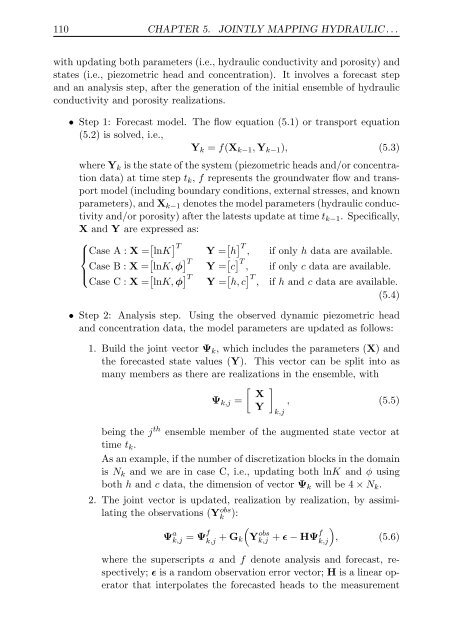
X <strong>and</strong> Y are expressed as:<br />
⎧<br />
⎪⎨ Case A : X = [ lnK ] T<br />
Y = [ h ] T<br />
, if only h data are available.<br />
Case B : X = [ lnK, ϕ ] T [ ] T<br />
Y = c , if only c data are available.<br />
⎪⎩<br />
Case C : X = [ lnK, ϕ ] T Y = [ h, c ] T , if h <strong>and</strong> c data are available.<br />
(5.4)<br />
• Step 2: Analysis step. Using the observed dynamic piezometric head<br />
<strong>and</strong> concentration data, the model parameters are updated as follows:<br />
1. Build the joint vector Ψk, which includes the parameters (X) <strong>and</strong><br />
the forecasted state values (Y). This vector can be split into as<br />
many members as there are realizations in the ensemble, with<br />
[ ]<br />
X<br />
Ψk,j = , (5.5)<br />
Y<br />
being the j th ensemble member <strong>of</strong> the augmented state vector at<br />
time tk.<br />
As an example, if the number <strong>of</strong> discretization blocks in the domain<br />
is Nk <strong>and</strong> we are in case C, i.e., updating both lnK <strong>and</strong> ϕ using<br />
both h <strong>and</strong> c data, the dimension <strong>of</strong> vector Ψk will be 4 × Nk.<br />
2. The joint vector is updated, realization by realization, by assimi-<br />
lating the observations (Y obs<br />
k ):<br />
Ψ a k,j<br />
= Ψf<br />
k,j + Gk<br />
k,j<br />
(<br />
Y obs<br />
)<br />
k,j + ϵ − HΨf k,j , (5.6)<br />
where the superscripts a <strong>and</strong> f denote analysis <strong>and</strong> forecast, respectively;<br />
ϵ is a r<strong>and</strong>om observation error vector; H is a linear operator<br />
that interpolates the forecasted heads to the measurement


