Upscaling and Inverse Modeling of Groundwater Flow and Mass ...

CHAPTER 4. MODELING TRANSIENT GROUNDWATER . . . 83
and cross-covariances involving conditioning points are zero, and so is the
Kalman gain at those locations; therefore, conductivities remain unchanged
through the entire Kalman filtering. In our case, after upscaling the finescale
conditional realizations, the resulting ensemble of hydraulic conductivity
tensor realizations will display smaller variances (through the ensemble) for
the tensors associated with interfaces close to the fine scale measurements
than for those far from the measurements. These smaller variances will result
in a smaller Kalman gain in the updating process at these locations, and
therefore will induce a soft conditioning of the interblock tensors on the fine
scale measurements.
The proposed method is implemented in the C software Upscaling-EnKF3D,
which is used in conjunction with the finite-difference program FLOWXYZ3D
(Li et al., 2010) in the forecasting step. From an operational point of view,
the proposed approach is suitable for parallel computation both in terms of
upscaling and EnKF, since each ensemble member is treated independently,
except for the computation of the Kalman gain.
4.3 Application Example
In this section, a synthetic experiment illustrates the effectiveness of the proposed
coupling of EnKF and upscaling.
4.3.1 Reference Field
We generate a realization of hydraulic conductivity over a domain discretized
into 350 by 350 cells of 1 m by 1 m using the code GCOSIM3D (Gómez-
Hernández and Journel, 1993).
We assume that, at this scale, conductivity is scalar and its natural logarithm,
lnK, can be characterized by a multiGaussian distribution of mean -5
(ln cm/s) and unit variance, with a strong anisotropic spatial correlation at
the 45 ◦ orientation. The correlation range in the largest continuity direction
(x ′ ) is λx ′ = 90 m and in the smallest continuity direction (y′ ) is λy ′ = 18 m.
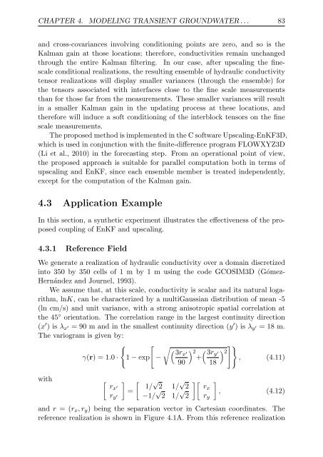
The variogram is given by:
{
γ(r) = 1.0 ·
with [ rx ′
ry ′
1 − exp
]
=
[
−
√ (3rx ′
90
[ 1/ √ 2 1/ √ 2
−1/ √ 2 1/ √ 2
) 2
+
][ rx
( 3ry ′
ry
18
]}
) 2
, (4.11)
]
, (4.12)
and r = (rx, ry) being the separation vector in Cartesian coordinates. The
reference realization is shown in Figure 4.1A. From this reference realization