Upscaling and Inverse Modeling of Groundwater Flow and Mass ...

86 CHAPTER 4. MODELING TRANSIENT GROUNDWATER . . .
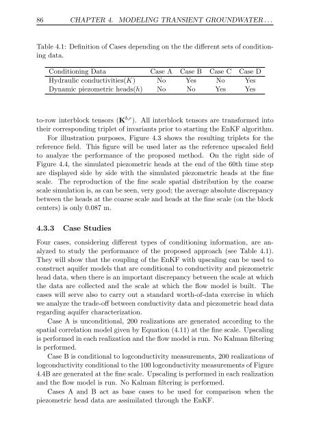
Table 4.1: Definition of Cases depending on the the different sets of conditioning
data.
Conditioning Data Case A Case B Case C Case D
Hydraulic conductivities(K) No Yes No Yes
Dynamic piezometric heads(h) No No Yes Yes
to-row interblock tensors (K b,r ). All interblock tensors are transformed into
their corresponding triplet of invariants prior to starting the EnKF algorithm.
For illustration purposes, Figure 4.3 shows the resulting triplets for the
reference field. This figure will be used later as the reference upscaled field
to analyze the performance of the proposed method. On the right side of
Figure 4.4, the simulated piezometric heads at the end of the 60th time step
are displayed side by side with the simulated piezometric heads at the fine
scale. The reproduction of the fine scale spatial distribution by the coarse
scale simulation is, as can be seen, very good; the average absolute discrepancy
between the heads at the coarse scale and heads at the fine scale (on the block
centers) is only 0.087 m.
4.3.3 Case Studies
Four cases, considering different types of conditioning information, are analyzed
to study the performance of the proposed approach (see Table 4.1).
They will show that the coupling of the EnKF with upscaling can be used to
construct aquifer models that are conditional to conductivity and piezometric
head data, when there is an important discrepancy between the scale at which
the data are collected and the scale at which the flow model is built. The
cases will serve also to carry out a standard worth-of-data exercise in which
we analyze the trade-off between conductivity data and piezometric head data
regarding aquifer characterization.
Case A is unconditional, 200 realizations are generated according to the
spatial correlation model given by Equation (4.11) at the fine scale. Upscaling
is performed in each realization and the flow model is run. No Kalman filtering
is performed.
Case B is conditional to logconductivity measurements, 200 realizations of
logconductivity conditional to the 100 logconductivity measurements of Figure
4.4B are generated at the fine scale. Upscaling is performed in each realization
and the flow model is run. No Kalman filtering is performed.
Cases A and B act as base cases to be used for comparison when the
piezometric head data are assimilated through the EnKF.