Upscaling and Inverse Modeling of Groundwater Flow and Mass ...

148 CHAPTER 6. GROUNDWATER FLOW INVERSE MODELING . . .
750
North
Training Image
.0
.0 East
750
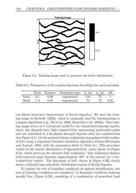
Figure 6.1: Training image used to generate the facies distribution.
Table 6.1: Parameters of the random functions describing the sand and shale
Mean Variance Variogram type λx [m] λy [m] sill
Sand 2.1 0.49 exponential 144 72 1
Shale -1.4 0.49 exponential 72 72 0.35
curvilinear structures characteristic of fluvial deposits.) We used the training
image in Strebelle (2002), which is commonly used for benchmarking to
compare algorithms (e.g., Wu et al., 2008; Mariethoz et al., 2010a). This training
image serves as a conceptual model for the channelized bimodal aquifer,
where the channels have high conductivities representing preferential paths
and are embedded in a floodplain fine-grid deposits with low conductivities
(see Figure 6.1); (ii) the generated facies realizations is populated with conductivities
using a sequential Gaussian simulation algorithm (Gómez-Hernández
and Journel, 1993) with the parameters listed in Table 6.1. This procedure
results in the spatial distribution of logconductivity values shown in Figure
6.2A, which serves as the reference lnK realization. This realization displays
well-connected sand channels (approximately 30% of the system) on a lowconductivity
matrix. The histogram of lnK, shown in Figure 6.2B, clearly
shows a bimodal logconductivity distribution typical of fluvial deposits.
To explore the role of boundary conditions on pattern identification, two
sets of boundary conditions are considered: (i) Boundary conditions inducing
parallel flow (Figure 6.3A), consisting of a combination of prescribed head
Sand
Shale