estudio y caracterización de un plasma de microondas a presión ...

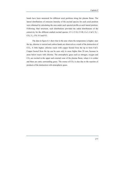
Capítulo 8
bands have been measured for different axial positions along the plasma flame. The
lateral distributions of emission intensity of the excited species for each axial position
were obtained by calculating the area under each spectral profile at each lateral position.
Following Abel inversion, such distributions provided the radial distributions of the
emissivity for the different studied excited species: Cl I, Cl II, Cl III, Cu I, CuCl, N2 + ,
CO2, C2, CN, O I and N I.
The data in figure 8.1 show that in the area where the temperature is higher, near
the tip, chlorine is ionized and carbon bands are observed as a result of the destruction of
CCl4. A little higher, chlorine reacts with copper booted from the tip to form CuCl.
Copper booted from the tip can be seen only in areas higher than 20 mm, because in
areas below reacts with chlorine. The atmospheric gases such as nitrogen, oxygen and
CO2 are excited in the upper and external zone of the plasma flame, where it is colder
and there are entry surrounding gases. The source of CO2 is also due to the reaction of
products of the destruction with atmospheric gases.
177