Cap. 4 Complejidad temporal de algoritmos - Inicio

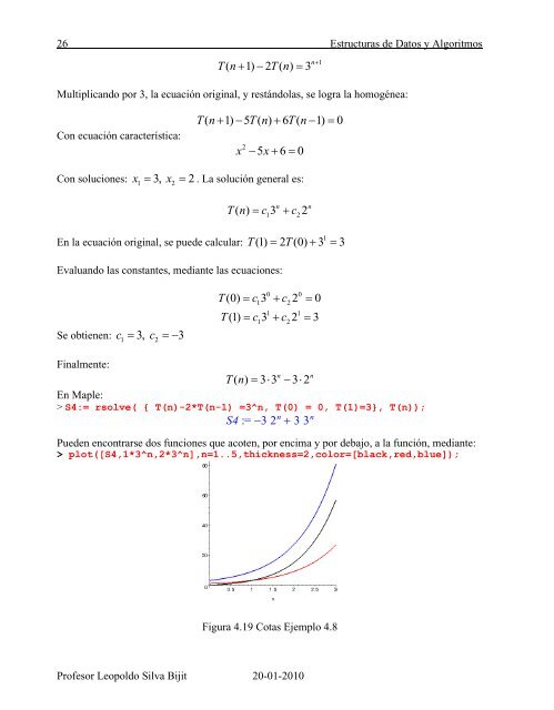
26 Estructuras de Datos y AlgoritmosT( n 1) 2 T( n) 3 n1Multiplicando por 3, la ecuación original, y restándolas, se logra la homogénea:Con ecuación característica:T( n 1) 5 T( n) 6 T( n 1) 0x25x 6 0Con soluciones: x1 3, x2 2 . La solución general es:T( n) c 3 c 2n1 2n1En la ecuación original, se puede calcular: T(1) 2 T(0) 3 3Evaluando las constantes, mediante las ecuaciones:Se obtienen: c1 3, c2 3T(0) c 3 c 2 00 01 2T (1) c 3 c 2 31 11 2Finalmente:n nTn ( ) 33 32En Maple:> S4:= rsolve( { T(n)-2*T(n-1) =3^n, T(0) = 0, T(1)=3}, T(n));S4 := 3 2 n 3 3 nPueden encontrarse dos funciones que acoten, por encima y por debajo, a la función, mediante:> plot([S4,1*3^n,2*3^n],n=1..5,thickness=2,color=[black,red,blue]);Figura 4.19 Cotas Ejemplo 4.8Profesor Leopoldo Silva Bijit 20-01-2010