- Page 1 and 2: Processing Modflow A Simulation Sys
- Page 3 and 4: 3.6.6 UCODE (Inverse Modeling) . ..
- Page 5 and 6: Preface Welcome to Processing Modfl
- Page 7 and 8: Processing Modflow 1 1. Introductio
- Page 9 and 10: Processing Modflow 3 the three-dime
- Page 11 and 12: Processing Modflow 5 Online Help Th
- Page 13 and 14: Processing Modflow 7 capture zone o
- Page 15 and 16: Processing Modflow 9 The first and
- Page 17 and 18: Processing Modflow 11 Now, you must
- Page 19 and 20: Processing Modflow 13 2. Repeat the
- Page 21 and 22: Processing Modflow 15 2. Choose Lea
- Page 23 and 24: Processing Modflow 17 simulation is
- Page 25 and 26: Processing Modflow 19 steps 3 to 5
- Page 27 and 28: Processing Modflow 21 Table 2.4 Out
- Page 29 and 30: Processing Modflow 23 results and u
- Page 31 and 32: Processing Modflow 25 Fig. 2.12 The
- Page 33 and 34: Processing Modflow 27 fields in the
- Page 35 and 36: Processing Modflow 29 Fig. 2.17 The
- Page 37 and 38: Processing Modflow 31 2.2 Simulatio
- Page 39 and 40: Processing Modflow 33 2. Click OK t
- Page 41 and 42: Processing Modflow 35 Fig. 2.24 The
- Page 43 and 44: Processing Modflow 37 Fig. 2.27 Sim
- Page 45 and 46: Processing Modflow 39 < To assign t
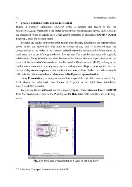
- Page 47: Processing Modflow 41 Fig. 2.32 The
- Page 51 and 52: Processing Modflow 45 Fig. 2.36 The
- Page 53 and 54: Processing Modflow 47 Note that PMW
- Page 55 and 56: Processing Modflow 49 the model dat
- Page 57 and 58: Processing Modflow 51 PMWIN will cr
- Page 59 and 60: Processing Modflow 53 Table 3.1 An
- Page 61 and 62: Processing Modflow 55 data and clic
- Page 63 and 64: Processing Modflow 57 Fig. 3.4 The
- Page 65 and 66: Processing Modflow 59 Fig. 3.5 The
- Page 67 and 68: Processing Modflow 61 3.2.2 The Zon
- Page 69 and 70: Processing Modflow 63 Fig. 3.9 The
- Page 71 and 72: Processing Modflow 65 Fig. 3.10 The
- Page 73 and 74: Processing Modflow 67 - Print: Prin
- Page 75 and 76: Processing Modflow 69 principal axe
- Page 77 and 78: Processing Modflow 71 Calculated, P
- Page 79 and 80: Processing Modflow 73 3.5 The Param
- Page 81 and 82: Processing Modflow 75 steady state
- Page 83 and 84: Processing Modflow 77 Vertical Hydr
- Page 85 and 86: Processing Modflow 79 3.6 The Model
- Page 87 and 88: Processing Modflow 81 RET ' RETM h>
- Page 89 and 90: Processing Modflow 83 boundaries be
- Page 91 and 92: Processing Modflow 85 For a confine
- Page 93 and 94: Processing Modflow 87 1. Recharge i
- Page 95 and 96: Processing Modflow 89 Leakage betwe
- Page 97 and 98: Processing Modflow 91 For the case
- Page 99 and 100:
Processing Modflow 93 < Parameter N
- Page 101 and 102:
Processing Modflow 95 MODFLOW < Tim
- Page 103 and 104:
Processing Modflow 97 MODFLOW < Wet
- Page 105 and 106:
Processing Modflow 99 well cell etc
- Page 107 and 108:
Processing Modflow 101 MODFLOW < So
- Page 109 and 110:
Processing Modflow 103 < Max. band
- Page 111 and 112:
Processing Modflow 105 < Allowed It
- Page 113 and 114:
Processing Modflow 107 MODFLOW < Ru
- Page 115 and 116:
Processing Modflow 109 Table 3.4 Ve
- Page 117 and 118:
Processing Modflow 111 MOC3D < Init
- Page 119 and 120:
Processing Modflow 113 MOC3D < Disp
- Page 121 and 122:
Processing Modflow 115 MOC3D < Stro
- Page 123 and 124:
Processing Modflow 117 Table 3.6 Na
- Page 125 and 126:
Processing Modflow 119 Fig. 3.40 Th
- Page 127 and 128:
Processing Modflow 121 higher numbe
- Page 129 and 130:
Processing Modflow 123 )t # Fixed p
- Page 131 and 132:
Processing Modflow 125 MT3D < Chemi
- Page 133 and 134:
Processing Modflow 127 beginning of
- Page 135 and 136:
Processing Modflow 129 < Misc.: - C
- Page 137 and 138:
Processing Modflow 131 3.6.4 MT3DMS
- Page 139 and 140:
Processing Modflow 133 < Weighting
- Page 141 and 142:
Processing Modflow 135 is infinite
- Page 143 and 144:
Processing Modflow 137 (ITER1): The
- Page 145 and 146:
Processing Modflow 139 3.6.5 PEST (
- Page 147 and 148:
Processing Modflow 141 define the e
- Page 149 and 150:
Processing Modflow 143 while s and
- Page 151 and 152:
Processing Modflow 145 - DERINCMUL:
- Page 153 and 154:
Processing Modflow 147 where N is t
- Page 155 and 156:
Processing Modflow 149 course of an
- Page 157 and 158:
Processing Modflow 151 PEST (Invers
- Page 159 and 160:
Processing Modflow 153 3.6.6 UCODE
- Page 161 and 162:
Processing Modflow 155 To define a
- Page 163 and 164:
Processing Modflow 157 < Options -
- Page 165 and 166:
Processing Modflow 159 Fig. 3.57 Th
- Page 167 and 168:
Processing Modflow 161 < To load an
- Page 169 and 170:
Processing Modflow 163 Use the Sear
- Page 171 and 172:
Processing Modflow 165 < Appearance
- Page 173 and 174:
Processing Modflow 167 - Ignore ina
- Page 175 and 176:
Processing Modflow 169 Maps... Fig.
- Page 177 and 178:
Processing Modflow 171 < Raster Gra
- Page 179 and 180:
Processing Modflow 173 4. The Advec
- Page 181 and 182:
Processing Modflow 175 where z 3 -1
- Page 183 and 184:
Processing Modflow 177 all velocity
- Page 185 and 186:
Processing Modflow 179 the cell ind
- Page 187 and 188:
Processing Modflow 181 Tool bar The
- Page 189 and 190:
Processing Modflow 183 The retardat
- Page 191 and 192:
Processing Modflow 185 small. Click
- Page 193 and 194:
Processing Modflow 187 < Contours:
- Page 195 and 196:
Processing Modflow 189 Particle Tra
- Page 197 and 198:
Processing Modflow 191 < Pathline C
- Page 199 and 200:
Processing Modflow 193 4.4 PMPATH O
- Page 201 and 202:
Processing Modflow 195 Particles To
- Page 203 and 204:
Processing Modflow 197 < To assign
- Page 205 and 206:
Processing Modflow 199 Where N is t
- Page 207 and 208:
Processing Modflow 201 EPA, and bey
- Page 209 and 210:
Processing Modflow 203 Fig. 5.5 Sea
- Page 211 and 212:
Processing Modflow 205 5.4 The Resu
- Page 213 and 214:
Processing Modflow 207 5.5 The Wate
- Page 215 and 216:
Processing Modflow 209 color of eac
- Page 217 and 218:
Processing Modflow 211 6. Examples
- Page 219 and 220:
Processing Modflow 213 Step1: Creat
- Page 221 and 222:
Processing Modflow 215 depth). Upon
- Page 223 and 224:
Processing Modflow 217 < To sepecif
- Page 225 and 226:
Processing Modflow 219 clicking wit
- Page 227 and 228:
Processing Modflow 221 5. In the Sa
- Page 229 and 230:
Processing Modflow 223 in this case
- Page 231 and 232:
Processing Modflow 225 Run transien
- Page 233 and 234:
Processing Modflow 227 6.1.2 Tutori
- Page 235 and 236:
Processing Modflow 229 3. Leave the
- Page 237 and 238:
Processing Modflow 231 < To specify
- Page 239 and 240:
Processing Modflow 233 Effective Po
- Page 241 and 242:
Processing Modflow 235 Step 6: Extr
- Page 243 and 244:
Processing Modflow 237 maximum numb
- Page 245 and 246:
Processing Modflow 239 distance fro
- Page 247 and 248:
Processing Modflow 241 6.2.2 Use of
- Page 249 and 250:
Processing Modflow 243 6.2.3 Simula
- Page 251 and 252:
Processing Modflow 245 Two steady-s
- Page 253 and 254:
Processing Modflow 247 down to the
- Page 255 and 256:
Processing Modflow 249 70 65 60 55
- Page 257 and 258:
Processing Modflow 251 Fig. 6.24 Hy
- Page 259 and 260:
Processing Modflow 253 6.2.6 Simula
- Page 261 and 262:
Processing Modflow 255 head or rive
- Page 263 and 264:
Processing Modflow 257 analytical s
- Page 265 and 266:
Processing Modflow 259 6.2.8 Simula
- Page 267 and 268:
Processing Modflow 261 and effectiv
- Page 269 and 270:
Processing Modflow 263 6.4 Automati
- Page 271 and 272:
Processing Modflow 265 Modeling App
- Page 273 and 274:
Processing Modflow 267 6.4.2 Estima
- Page 275 and 276:
Processing Modflow 269 6.4.3 The Th
- Page 277 and 278:
Processing Modflow 271 Fig. 6.40 Dr
- Page 279 and 280:
Processing Modflow 273 Fig. 6.41 Co
- Page 281 and 282:
Processing Modflow 275 6.5 Geotechn
- Page 283 and 284:
Processing Modflow 277 6.5.2 Flow N
- Page 285 and 286:
Processing Modflow 279 6.5.3 Seepag
- Page 287 and 288:
Processing Modflow 281 Fig. 6.51 Ca
- Page 289 and 290:
Processing Modflow 283 3 penetrated
- Page 291 and 292:
Processing Modflow 285 6.5.5 Compac
- Page 293 and 294:
Processing Modflow 287 Fig. 6.57 Di
- Page 295 and 296:
Processing Modflow 289 irreversible
- Page 297 and 298:
Processing Modflow 291 (Rausch, 199
- Page 299 and 300:
Processing Modflow 293 6.6.3 Benchm
- Page 301 and 302:
Processing Modflow 295 6.7 Miscella
- Page 303 and 304:
Processing Modflow 297 Fig. 6.65 Co
- Page 305 and 306:
Processing Modflow 299 6.7.2 An Exa
- Page 307 and 308:
Processing Modflow 301 7. Appendice
- Page 309 and 310:
Processing Modflow 303 COLOR is the
- Page 311 and 312:
Processing Modflow 305 The unit of
- Page 313 and 314:
Processing Modflow 307 Appendix 3:
- Page 315 and 316:
Processing Modflow 309 PEST Instruc
- Page 317 and 318:
Processing Modflow 311 YLZ ZONE Spe
- Page 319 and 320:
Processing Modflow 313 STC CBC Stre
- Page 321 and 322:
Processing Modflow 315 961...990 ZO
- Page 323 and 324:
Processing Modflow 317 Table 7.2 IU
- Page 325 and 326:
Processing Modflow 319 8. Reference
- Page 327 and 328:
Processing Modflow 321 Franke, R. (
- Page 329 and 330:
Processing Modflow 323 Leake, S.A.
- Page 331:
Processing Modflow 325 Shepard, D.,