Onto.PT: Towards the Automatic Construction of a Lexical Ontology ...

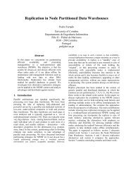
102 Chapter 6. Thesaurus Enrichment
Measure Mode σ Sets/Pair P R RR F1 RF1 F0.5 RF0.5
All – – 4.31 0.37 1.00 1.00 0.54 0.54 0.42 0.42
Best
0.00
0.15
1.07
0.52
0.63
0.72
0.49
0.25
0.81
0.45
0.55
0.37
0.71
0.56
0.59
0.53
0.66
0.65
Jaccard
All
0.05
0.1
0.15
3.14
1.52
0.77
0.45
0.59
0.70
0.86
0.52
0.33
0.96
0.69
0.48
0.59
0.55
0.45
0.61
0.63
0.57
0.49
0.57
0.57
0.50
0.61
0.64
0.2 0.41 0.78 0.20 0.32 0.32 0.46 0.50 0.61
Best
0.00
0.15
1.06
1.04
0.63
0.64
0.48
0.47
0.81
0.80
0.55
0.54
0.71
0.71
0.60
0.60
0.66
0.67
0.1 3.98 0.39 0.96 0.98 0.55 0.56 0.44 0.44
Overlap
All
0.4
0.45
0.5
1.28
1.05
0.88
0.63
0.67
0.70
0.44
0.37
0.32
0.61
0.53
0.48
0.52
0.47
0.44
0.62
0.59
0.57
0.58
0.57
0.57
0.63
0.63
0.64
0.55 0.65 0.74 0.25 0.37 0.37 0.50 0.53 0.62
0.6 0.50 0.79 0.19 0.31 0.30 0.45 0.48 0.60
Best
0.00
0.15
1.06
0.87
0.63
0.64
0.49
0.45
0.81
0.7
0.55
0.53
0.71
0.67
0.60
0.59
0.66
0.65
0.1 2.97 0.46 0.85 0.95 0.60 0.62 0.51 0.51
Dice
All
0.15
0.2
0.25
2.00
1.26
0.81
0.54
0.62
0.71
0.65
0.45
0.35
0.80
0.63
0.50
0.59
0.52
0.47
0.64
0.62
0.59
0.56
0.57
0.59
0.58
0.62
0.66
0.3 0.55 0.77 0.25 0.38 0.38 0.51 0.54 0.64
0.35 0.35 0.81 0.16 0.27 0.26 0.41 0.44 0.58
Best
0.00
0.15
1.05
0.94
0.64
0.66
0.48
0.45
0.81
0.75
0.55
0.53
0.71
0.70
0.60
0.60
0.66
0.68
0.1 3.34 0.44 0.89 0.97 0.59 0.60 0.49 0.49
0.15 2.40 0.52 0.75 0.88 0.61 0.66 0.55 0.57
Cosine
0.2 1.58 0.58 0.53 0.70 0.55 0.64 0.57 0.60
All 0.25 1.08 0.66 0.41 0.58 0.51 0.61 0.59 0.64
0.3 0.74 0.74 0.32 0.48 0.45 0.58 0.59 0.67
0.35 0.48 0.82 0.21 0.35 0.34 0.49 0.52 0.64
0.4 0.32 0.80 0.15 0.25 0.25 0.37 0.43 0.55
Table 6.3: Evaluation against intersection of annotators 1 and 2.
1. Create a new sparse matrix M(|V | × |V |).
2. In each cell Mij, put the similarity between the adjacency vectors of the word
in vi with the adjacency vectors of vj, Mij = sim(vi, vj);
3. Extract a cluster Ci from each row Mi, consisting of the words vj where Mij > θ,
a selected threshold. A lower θ leads to larger synsets and higher ambiguity,
while a larger θ will result on less and smaller synsets or no synsets at all.
4. For each cluster Ci with all elements included in a larger cluster Cj (Ci∪Cj = Cj
and Ci ∩ Cj = Ci), Ci and Cj are merged, giving rise to a new cluster Ck with
the same elements of Cj.
After clustering, we will have a thesaurus T with synsets Si and a set of discovered
clusters C. A simple thing to do would be to handle the clusters as synsets and add
then to the thesaurus. However, some of the clusters might be already included or
partly included in existing synsets. Therefore, before adding the clusters to T , we
compute the similarity between the words in each synset Si and the words in each
discovered cluster Cj. For this purpose, we measure the overlap between the former
sets, using the overlap coefficient:
Overlap(Si, Cj) =
|Si ∩ C ||
min(|Si|, |Cj|)
(6.1)