Soner Bekleric Title of Thesis: Nonlinear Prediction via Volterra Ser
Soner Bekleric Title of Thesis: Nonlinear Prediction via Volterra Ser
Soner Bekleric Title of Thesis: Nonlinear Prediction via Volterra Ser

Create successful ePaper yourself
Turn your PDF publications into a flip-book with our unique Google optimized e-Paper software.
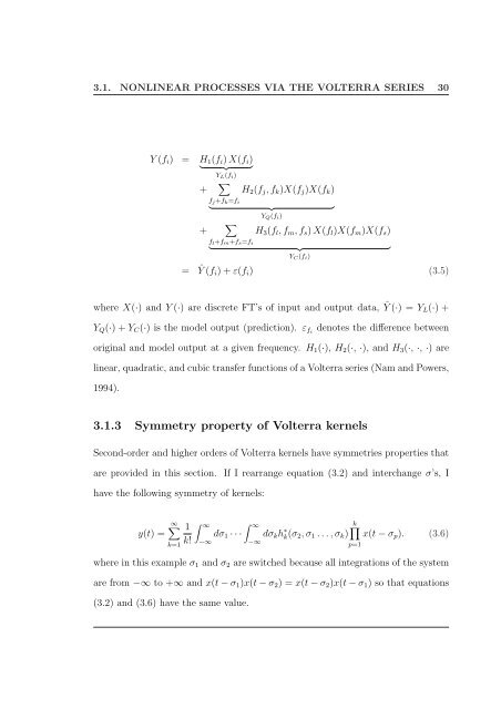
3.1. NONLINEAR PROCESSES VIA THE VOLTERRA SERIES 30<br />
Y (fi) = H1(fi) X(fi)<br />
<br />
+<br />
YL(fi)<br />
<br />
H2(fj, fk)X(fj)X(fk)<br />
+<br />
fj+fk=fi<br />
<br />
YQ(fi)<br />
<br />
H3(fl, fm, fs) X(fl)X(fm)X(fs)<br />
fl+fm+fs=fi<br />
<br />
YC(fi)<br />
<br />
= ˆ Y (fi) + ε(fi) (3.5)<br />
where X(·) and Y (·) are discrete FT’s <strong>of</strong> input and output data, ˆ Y (·) = YL(·) +<br />
YQ(·) + YC(·) is the model output (prediction). εfi<br />
denotes the difference between<br />
original and model output at a given frequency. H1(·), H2(·, ·), and H3(·, ·, ·) are<br />
linear, quadratic, and cubic transfer functions <strong>of</strong> a <strong>Volterra</strong> series (Nam and Powers,<br />
1994).<br />
3.1.3 Symmetry property <strong>of</strong> <strong>Volterra</strong> kernels<br />
Second-order and higher orders <strong>of</strong> <strong>Volterra</strong> kernels have symmetries properties that<br />
are provided in this section. If I rearrange equation (3.2) and interchange σ’s, I<br />
have the following symmetry <strong>of</strong> kernels:<br />
y(t) =<br />
∞<br />
k=1<br />
<br />
1 ∞ ∞<br />
dσ1 · · ·<br />
k! −∞<br />
−∞<br />
dσkh ∗ k<br />
k(σ2, σ1 . . . , σk)<br />
p=1<br />
x(t − σp). (3.6)<br />
where in this example σ1 and σ2 are switched because all integrations <strong>of</strong> the system<br />
are from −∞ to +∞ and x(t − σ1)x(t − σ2) = x(t − σ2)x(t − σ1) so that equations<br />
(3.2) and (3.6) have the same value.