Soner Bekleric Title of Thesis: Nonlinear Prediction via Volterra Ser
Soner Bekleric Title of Thesis: Nonlinear Prediction via Volterra Ser
Soner Bekleric Title of Thesis: Nonlinear Prediction via Volterra Ser
You also want an ePaper? Increase the reach of your titles
YUMPU automatically turns print PDFs into web optimized ePapers that Google loves.
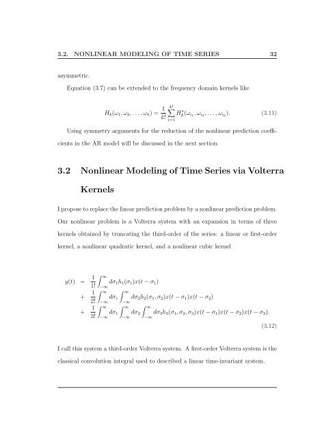
3.2. NONLINEAR MODELING OF TIME SERIES 32<br />
asymmetric.<br />
Equation (3.7) can be extended to the frequency domain kernels like<br />
Hk(ω1, ω2, . . . , ωk) = 1<br />
k!<br />
k!<br />
i=1<br />
H ∗ k(ωi1, ωi2, . . . , ωik ). (3.11)<br />
Using symmetry arguments for the reduction <strong>of</strong> the nonlinear prediction coeffi-<br />
cients in the AR model will be discussed in the next section.<br />
3.2 <strong>Nonlinear</strong> Modeling <strong>of</strong> Time <strong>Ser</strong>ies <strong>via</strong> <strong>Volterra</strong><br />
Kernels<br />
I propose to replace the linear prediction problem by a nonlinear prediction problem.<br />
Our nonlinear problem is a <strong>Volterra</strong> system with an expansion in terms <strong>of</strong> three<br />
kernels obtained by truncating the third-order <strong>of</strong> the series: a linear or first-order<br />
kernel, a nonlinear quadratic kernel, and a nonlinear cubic kernel<br />
y(t) = 1<br />
∞<br />
1!<br />
+ 1<br />
2!<br />
+ 1<br />
3!<br />
−∞<br />
∞<br />
dσ1h1(σ1)x(t − σ1)<br />
dσ1<br />
−∞<br />
∞<br />
dσ1<br />
−∞<br />
∞<br />
−∞<br />
∞<br />
dσ2h2(σ1, σ2)x(t − σ1)x(t − σ2)<br />
dσ2<br />
−∞<br />
∞<br />
−∞<br />
dσ3h3(σ1, σ2, σ3)x(t − σ1)x(t − σ2)x(t − σ3).<br />
(3.12)<br />
I call this system a third-order <strong>Volterra</strong> system. A first-order <strong>Volterra</strong> system is the<br />
classical convolution integral used to described a linear time-invariant system.


