Hi-Res PDF - CRCnetBASE

Longitudinal Train Dynamics 273
Resistance, N/tonne
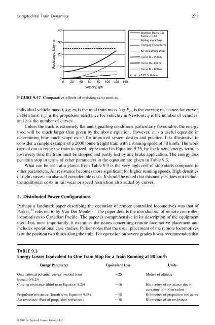
individual vehicle mass i ,kg; m t is the total train mass, kg; F crj is the curving resistance for curve j
in Newtons; F pri is the propulsion resistance for vehicle i in Newtons; q is the number of vehicles;
and r is the number of curves.
Unless the track is extremely flat and signalling conditions particularly favourable, the energy
used will be much larger than given bythe above equation. However, it is auseful equation in
determining how much scope exists for improved system design and practice. It is illustrative to
consider asimple example of a2000tonne freight train with arunning speed of 80 km/h. The work
carried out to bring the train to speed, represented in Equation 9.25, by the kinetic energy term, is
lost every time the train must be stopped and partly lost by any brake application. The energy loss
per train stop in terms of other parameters in the equation are given inTable 9.3.
What can be seen at aglance from Table 9.3 is the very high cost of stop starts compared to
other parameters. Air resistance becomes more significant for higherrunning speeds. High densities
of tight curves can also add considerablecosts. It shouldbenoted that this analysisdoes not include
the additional costs in rail wear or speed restriction also added by curves.
5. Distributed Power Configurations
40
30
20
10
0
0 20 40 60 80 100 120 140
Velocity, kph
FIGURE 9.47 Comparative effects of resistances to motion.
Modified Davis Car
Factor =0.85
Rolling stockTerm
Flanging FactorTerm
Air ResistanceTerm
Curve R=200 m
Curve R= 400 m
Curve R=800 m
0.25 %Grade
Perhaps alandmark paper describing the operation of remote controlled locomotives was that of
Parker, 22 referred to by Van Der Meulen. 3 The paper details the introduction of remote controlled
locomotives to Canadian Pacific. The paper is comprehensive in its description of the equipment
used, but, most importantly, it examines the issues concerning remote locomotive placement and
includes operational case studies. Parker notes that the usual placement of the remote locomotives
is at the position two thirds alongthe train. For operation on severe grades it was recommended that
TABLE 9.3
Energy Losses Equivalent to One Train Stop for aTrain Running at 80 km/h
Energy Parameter Equivalent Loss Units
Gravitational potential energy (second term
Equation 9.25)
, 25 Metres of altitude
Curving resistance (third term Equation 9.25) , 16 Kilometres ofresistance due to
curvature of400 mradius
Propulsion resistance (fourth term Equation 9.25) , 18 Kilometres ofpropulsion resistance
Air resistance (Part of propulsion resistance) , 38 Kilometres ofair resistance
© 2006 by Taylor & Francis Group, LLC