Numerical Methods Course Notes Version 0.1 (UCSD Math 174, Fall ...
Numerical Methods Course Notes Version 0.1 (UCSD Math 174, Fall ...
Numerical Methods Course Notes Version 0.1 (UCSD Math 174, Fall ...
You also want an ePaper? Increase the reach of your titles
YUMPU automatically turns print PDFs into web optimized ePapers that Google loves.
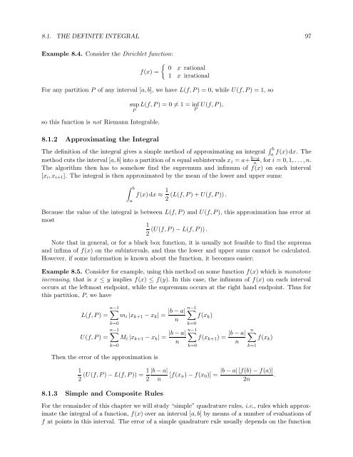
8.1. THE DEFINITE INTEGRAL 97<br />
Example 8.4. Consider the Dirichlet function:<br />
{ 0 x rational<br />
f(x) =<br />
1 x irrational<br />
For any partition P of any interval [a, b], we have L(f, P ) = 0, while U(f, P ) = 1, so<br />
so this function is not Riemann Integrable.<br />
8.1.2 Approximating the Integral<br />
sup L(f, P ) = 0 ≠ 1 = inf U(f, P ),<br />
P<br />
P<br />
The definition of the integral gives a simple method of approximating an integral ∫ b<br />
a<br />
f(x) dx. The<br />
method cuts the interval [a, b] into a partition of n equal subintervals x i = a+ b−a<br />
n<br />
, for i = 0, 1, . . . , n.<br />
The algorithm then has to somehow find the supremum and infimum of f(x) on each interval<br />
[x i , x i+1 ]. The integral is then approximated by the mean of the lower and upper sums:<br />
∫ b<br />
a<br />
f(x) dx ≈ 1 (L(f, P ) + U(f, P )) .<br />
2<br />
Because the value of the integral is between L(f, P ) and U(f, P ), this approximation has error at<br />
most<br />
1<br />
(U(f, P ) − L(f, P )) .<br />
2<br />
Note that in general, or for a black box function, it is usually not feasible to find the suprema<br />
and infima of f(x) on the subintervals, and thus the lower and upper sums cannot be calculated.<br />
However, if some information is known about the function, it becomes easier:<br />
Example 8.5. Consider for example, using this method on some function f(x) which is monotone<br />
increasing, that is x ≤ y implies f(x) ≤ f(y). In this case, the infimum of f(x) on each interval<br />
occurs at the leftmost endpoint, while the supremum occurs at the right hand endpoint. Thus for<br />
this partition, P, we have<br />
n−1<br />
∑<br />
L(f, P ) = m i |x k+1 − x k | =<br />
k=0<br />
n−1<br />
∑<br />
U(f, P ) = M i |x k+1 − x k | =<br />
k=0<br />
|b − a|<br />
n<br />
|b − a|<br />
n<br />
n−1<br />
∑<br />
f(x k )<br />
k=0<br />
n−1<br />
∑<br />
f(x k+1 ) =<br />
k=0<br />
|b − a|<br />
n<br />
n∑<br />
f(x k )<br />
k=1<br />
Then the error of the approximation is<br />
1<br />
2 (U(f, P ) − L(f, P )) = 1 |b − a|<br />
[f(x n ) − f(x 0 )] =<br />
2 n<br />
8.1.3 Simple and Composite Rules<br />
|b − a| [f(b) − f(a)]<br />
.<br />
2n<br />
For the remainder of this chapter we will study “simple” quadrature rules, i.e., rules which approximate<br />
the integral of a function, f(x) over an interval [a, b] by means of a number of evaluations of<br />
f at points in this interval. The error of a simple quadrature rule usually depends on the function


