Numerical Methods Course Notes Version 0.1 (UCSD Math 174, Fall ...

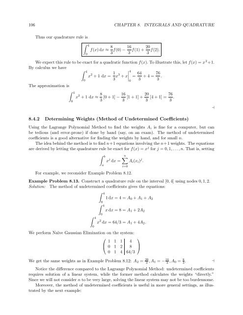
106 CHAPTER 8. INTEGRALS AND QUADRATURE
Thus our quadrature rule is
∫ 4
0
f(x) dx ≈ 8 16
f(0) −
3 3 f(1) + 20 3 f(2).
We expect this rule to be exact for a quadratic function f(x). To illustrate this, let f(x) = x 2 +1.
By calculus we have
∫ 4
x 2 + 1 dx = 1 4
3 x3 + x
∣ = 64
3 + 4 = 76 3 .
The approximation is
∫ 4
0
0
x 2 + 1 dx ≈ 8 3 [0 + 1] − 16 3
0
[1 + 1] +
20
3 [4 + 1] = 76 3 . ⊣
8.4.2 Determining Weights (Method of Undetermined Coefficients)
Using the Lagrange Polynomial Method to find the weights A i is fine for a computer, but can
be tedious (and error-prone) if done by hand (say, on an exam). The method of undetermined
coefficients is a good alternative for finding the weights by hand, and for small n.
The idea behind the method is to find n+1 equations involving the n+1 weights. The equations
are derived by letting the quadrature rule be exact for f(x) = x j for j = 0, 1, . . . , n. That is, setting
∫ b
a
x j dx =
n∑
A i (x i ) j .
i=0
For example, we reconsider Example Problem 8.12.
Example Problem 8.13. Construct a quadrature rule on the interval [0, 4] using nodes 0, 1, 2.
Solution: The method of undetermined coefficients gives the equations:
∫ 4
0
∫ 4
0
∫ 4
0
1 dx = 4 = A 0 + A 1 + A 2
x dx = 8 = A 1 + 2A 2
x 2 dx = 64/3 = A 1 + 4A 2 .
We perform Naïve Gaussian Elimination on the system:
⎛
1 1 1 4
⎞
⎝ 0 1 2 8 ⎠
0 1 4 64/3
We get the same weights as in Example Problem 8.12: A 2 = 20
3 , A 1 = − 16 3 , A 0 = 8 3 . ⊣
Notice the difference compared to the Lagrange Polynomial Method: undetermined coefficients
requires solution of a linear system, while the former method calculates the weights “directly.”
Since we will not consider n to be very large, solving the linear system may not be too burdensome.
Moreover, the method of undetermined coefficients is useful in more general settings, as illustrated
by the next example: