Numerical Methods Course Notes Version 0.1 (UCSD Math 174, Fall ...

3.4. ITERATIVE SOLUTIONS 37
3.4.2 Dividing by Multiplying
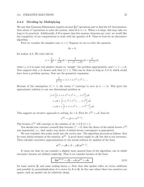
We saw that Gaussian Elimination requires around 2 3 n3 operations just to find the LU factorization,
then about n 2 operations to solve the system, when A is n × n. When n is large, this may take too
long to be practical. Additionally, if A is sparse (has few nonzero elements per row), we would like
the complexity of our computations to scale with the sparsity of A. Thus we look for an alternative
algorithm.
First we consider the simplest case, n = 1. Suppose we are to solve the equation
for scalars A, b. We solve this by
Ax = b.
x = 1 A b = 1
ωA ωb = 1
1 − (1 − ωA) ωb = 1
1 − r ωb,
where ω ≠ 0 is some real number chosen to “weight” the problem appropriately, and r = 1 − ωA.
Now suppose that ω is chosen such that |r| < 1. This can be done so long as A ≠ 0, which would
have been a problem anyway. Now use the geometric expansion:
1
1 − r = 1 + r + r2 + r 3 + . . .
Because of the assumption |r| < 1, the terms r n converge to zero as n → ∞. This gives the
approximate solution to our one dimensional problem as
[
x ≈ 1 + r + r 2 + r 3 + . . . + r k] ωb
[
= ωb + r + r 2 + r 3 + . . . + r k] ωb
[
= ωb + r 1 + r + r 2 + . . . + r k−1] ωb
This suggests an iterative approach to solving Ax = b. First let x (0) = ωb, then let
x (k) = ωb + rx (k−1) .
The iterates x (k) will converge to the solution of Ax = b if |r| < 1.
You should now convince yourself that because r n → 0, that the choice of the initial iterate x (0)
was immaterial, i.e., that under any choice of initial iterate convergence is guaranteed.
We now translate this scalar result into the vector case. The algorithm proceeds as follows: first
fix some initial estimate of the solution, x (0) . A good choice might be ωb, but this is not necessary.
Then calculate successive approximations to the actual solution by updates of the form
x (k) = ωb + (I − ωA) x (k−1) .
It turns out that we can consider a slightly more general form of the algorithm, one in which
successive iterates are defined implicitly. That is we consider iterates of the form
Qx (k+1) = (Q − ωA) x (k) + ωb, (3.3)
for some matrix Q, and some scaling factor ω. Note that this update relies on vector additions
and possibly by premultiplication of a vector by A or Q. In the case where these two matrices are
sparse, such an update can be relatively cheap.