Numerical Methods Course Notes Version 0.1 (UCSD Math 174, Fall ...

5.1. POLYNOMIAL INTERPOLATION 63
2
l0(x)
l1(x)
l2(x)
1.5
1
0.5
0
-0.5
-1
0 0.5 1 1.5 2 2.5 3 3.5
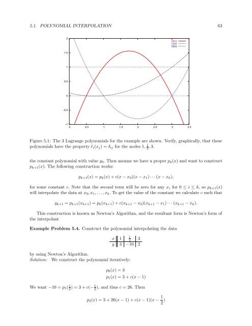
Figure 5.1: The 3 Lagrange polynomials for the example are shown. Verify, graphically, that these
polynomials have the property l i (x j ) = δ ij for the nodes 1, 1 2 , 3.
the constant polynomial with value y 0 . Then assume we have a proper p k (x) and want to construct
p k+1 (x). The following construction works:
p k+1 (x) = p k (x) + c(x − x 0 )(x − x 1 ) · · · (x − x k ),
for some constant c. Note that the second term will be zero for any x i for 0 ≤ i ≤ k, so p k+1 (x)
will interpolate the data at x 0 , x 1 , . . . , x k . To get the value of the constant we calculate c such that
y k+1 = p k+1 (x k+1 ) = p k (x k+1 ) + c(x k+1 − x 0 )(x k+1 − x 1 ) · · · (x k+1 − x k ).
This construction is known as Newton’s Algorithm, and the resultant form is Newton’s form of
the interpolant
Example Problem 5.4. Construct the polynomial interpolating the data
x 1
1
2
3
y 3 −10 2
by using Newton’s Algorithm.
Solution: We construct the polynomial iteratively:
p 0 (x) = 3
p 1 (x) = 3 + c(x − 1)
We want −10 = p 1 ( 1 2 ) = 3 + c(− 1 2
), and thus c = 26. Then
p 2 (x) = 3 + 26(x − 1) + c(x − 1)(x − 1 2 )