Numerical Methods Course Notes Version 0.1 (UCSD Math 174, Fall ...

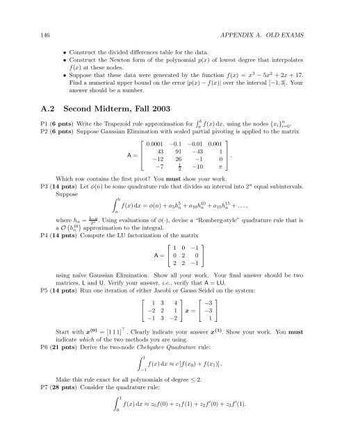
146 APPENDIX A. OLD EXAMS
• Construct the divided differences table for the data.
• Construct the Newton form of the polynomial p(x) of lowest degree that interpolates
f(x) at these nodes.
• Suppose that these data were generated by the function f(x) = x 3 − 5x 2 + 2x + 17.
Find a numerical upper bound on the error |p(x) − f(x)| over the interval [−1, 3]. Your
answer should be a number.
A.2 Second Midterm, Fall 2003
P1 (6 pnts) Write the Trapezoid rule approximation for ∫ b
a f(x) dx, using the nodes {x i} n i=0 .
P2 (6 pnts) Suppose Gaussian Elimination with scaled partial pivoting is applied to the matrix
A =
⎡
⎢
⎣
0.0001 −0.1 −0.01 0.001
43 91 −43 1
−12 26 −1 0
1
−7
2
−10 π
Which row contains the first pivot? You must show your work.
P3 (14 pnts) Let φ(n) be some quadrature rule that divides an interval into 2 n equal subintervals.
Suppose
∫ b
a
⎤
⎥
⎦ .
f(x) dx = φ(n) + a 5 h 5 n + a 10 h 10
n + a 15 h 15
n + . . . ,
where h n = b−a
2
. Using evaluations of φ(·), devise a “Romberg-style” quadrature rule that is
n
a O ( h 10 )
n approximation to the integral.
P4 (14 pnts) Compute the LU factorization of the matrix
⎡
1 0
⎤
−1
A = ⎣ 0 2 0 ⎦
2 2 −1
using naïve Gaussian Elimination. Show all your work. Your final answer should be two
matrices, L and U. Verify your answer, i.e., verify that A = LU.
P5 (14 pnts) Run one iteration of either Jacobi or Gauss Seidel on the system:
⎡
⎣
1 3 4
−2 2 1
−1 3 −2
⎤
⎡
⎦ x = ⎣
Start with x (0) = [1 1 1] ⊤ . Clearly indicate your answer x (1) . Show your work. You must
indicate which of the two methods you are using.
P6 (21 pnts) Derive the two-node Chebyshev Quadrature rule:
∫ 1
−1
−3
−3
1
⎤
⎦
f(x) dx ≈ c [f(x 0 ) + f(x 1 )] .
Make this rule exact for all polynomials of degree ≤ 2.
P7 (28 pnts) Consider the quadrature rule:
∫ 1
0
f(x) dx ≈ z 0 f(0) + z 1 f(1) + z 2 f ′ (0) + z 3 f ′ (1).