Numerical Methods Course Notes Version 0.1 (UCSD Math 174, Fall ...

3.4. ITERATIVE SOLUTIONS 39
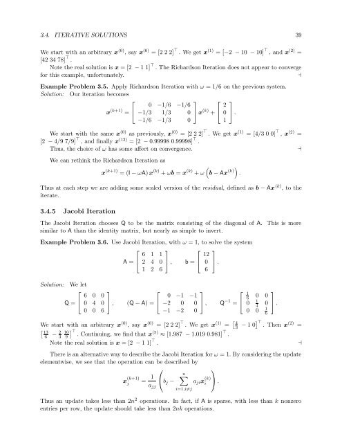
We start with an arbitrary x (0) , say x (0) = [2 2 2] ⊤ . We get x (1) = [−2 − 10 − 10] ⊤ , and x (2) =
[42 34 78] ⊤ .
Note the real solution is x = [2 − 1 1] ⊤ . The Richardson Iteration does not appear to converge
for this example, unfortunately.
⊣
Example Problem 3.5. Apply Richardson Iteration with ω = 1/6 on the previous system.
Solution: Our iteration becomes
⎡
⎤ ⎡ ⎤
0 −1/6 −1/6
2
x (k+1) = ⎣ −1/3 1/3 0 ⎦ x (k) + ⎣ 0 ⎦ .
−1/6 −1/3 0
1
We start with the same x (0) as previously, x (0) = [2 2 2] ⊤ . We get x (1) = [4/3 0 0] ⊤ , x (2) =
[2 − 4/9 7/9] ⊤ , and finally x (12) = [2 − 0.99998 0.99998] ⊤ .
Thus, the choice of ω has some affect on convergence.
⊣
We can rethink the Richardson Iteration as
x (k+1) = (I − ωA) x (k) + ωb = x (k) + ω
(
b − Ax (k)) .
Thus at each step we are adding some scaled version of the residual, defined as b − Ax (k) , to the
iterate.
3.4.5 Jacobi Iteration
The Jacobi Iteration chooses Q to be the matrix consisting of the diagonal of A. This is more
similar to A than the identity matrix, but nearly as simple to invert.
Example Problem 3.6. Use Jacobi Iteration, with ω = 1, to solve the system
⎡
6 1
⎤
1
⎡ ⎤
12
A = ⎣ 2 4 0 ⎦ , b = ⎣ 0 ⎦ .
1 2 6
6
Solution: We let
⎡
6 0
⎤
0
⎡
Q = ⎣ 0 4 0 ⎦ , (Q − A) = ⎣
0 0 6
0 −1 −1
−2 0 0
−1 −2 0
⎤
⎡
⎦ , Q −1 = ⎣
1
6
0 0
1
0
4
0
0 0
1
6
⎤
⎦ .
We start with an arbitrary x (0) , say x (0) = [2 2 2] ⊤ . We get x (1) = [ 4
3 − 1 0] ⊤ . Then x (2) =
[ 13
6
− 2 ]
10 ⊤
3 9 . Continuing, we find that x (5) ≈ [1.987 − 1.019 0.981] ⊤ .
Note the real solution is x = [2 − 1 1] ⊤ .
⊣
There is an alternative way to describe the Jacobi Iteration for ω = 1. By considering the update
elementwise, we see that the operation can be described by
⎛
⎞
x (k+1)
j
= 1
n∑
⎝b j − a ji x (k) ⎠
i
.
a jj
i=1,i≠j
Thus an update takes less than 2n 2 operations. In fact, if A is sparse, with less than k nonzero
entries per row, the update should take less than 2nk operations.