Numerical Methods Course Notes Version 0.1 (UCSD Math 174, Fall ...

12 CHAPTER 2. A “CRASH” COURSE IN OCTAVE/MATLAB
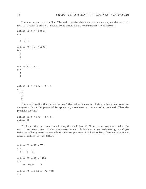
You now have a command line. The basic octavian data structure is a matrix; a scalar is a 1×1
matrix, a vector is an n × 1 matrix. Some simple matrix constructions are as follows:
octave:2> a = [1 2 3]
a =
1 2 3
octave:3> b = [5;4;3]
b =
5
4
3
octave:4> c = a’
c =
1
2
3
octave:5> d = 5*c - 2 * b
d =
-5
2
9
You should notice that octave “echoes” the lvalues it creates. This is either a feature or an
annoyance. It can be prevented by appending a semicolon at the end of a command. Thus the
previous becomes
octave:5> d = 5*c - 2 * b;
octave:6>
For illustration purposes, I am leaving the semicolon off. To access an entry or entries of a
matrix, use parentheses. In the case where the variable is a vector, you only need give a single
index, as follows; when the variable is a matrix, you need give both indices. You can also give a
range of indices, as what follows:
octave:6> a(1) = 77
a =
77 2 3
octave:7> a(2) = -400
a =
77 -400 3
octave:8> a(2:3) = [22 333]
a =