- Page 1: Numerical Methods Course Notes Vers
- Page 5 and 6: Contents Acknowledgments i 1 Introd
- Page 7 and 8: CONTENTS v 8 Integrals and Quadratu
- Page 9 and 10: Chapter 1 Introduction 1.1 Taylor
- Page 11 and 12: 1.1. TAYLOR’S THEOREM 3 with the
- Page 13 and 14: 1.3. EIGENVALUES 5 To correct this
- Page 15 and 16: 1.3. EIGENVALUES 7 Example Problem
- Page 17 and 18: 1.3. EIGENVALUES 9 for all vectors
- Page 19 and 20: Chapter 2 A “Crash” Course in o
- Page 21 and 22: 2.1. GETTING STARTED 13 77 22 333 o
- Page 23 and 24: 2.2. USEFUL COMMANDS 15 octave:22>
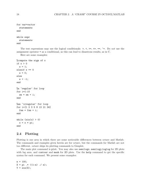
- Page 25: 2.3. PROGRAMMING AND CONTROL 17 x1
- Page 29 and 30: 2.4. PLOTTING 21 Exercises (2.1) Wh
- Page 31 and 32: Chapter 3 Solving Linear Systems A
- Page 33 and 34: 3.1. GAUSSIAN ELIMINATION WITH NAÏ
- Page 35 and 36: 3.2. PIVOTING STRATEGIES FOR GAUSSI
- Page 37 and 38: 3.2. PIVOTING STRATEGIES FOR GAUSSI
- Page 39 and 40: 3.3. LU FACTORIZATION 31 appropriat
- Page 41 and 42: 3.3. LU FACTORIZATION 33 We pivot o
- Page 43 and 44: 3.4. ITERATIVE SOLUTIONS 35 3.3.3 S
- Page 45 and 46: 3.4. ITERATIVE SOLUTIONS 37 3.4.2 D
- Page 47 and 48: 3.4. ITERATIVE SOLUTIONS 39 We star
- Page 49 and 50: 3.4. ITERATIVE SOLUTIONS 41 Now not
- Page 51 and 52: 3.4. ITERATIVE SOLUTIONS 43 Remembe
- Page 53 and 54: 3.4. ITERATIVE SOLUTIONS 45 is the
- Page 55 and 56: Chapter 4 Finding Roots 4.1 Bisecti
- Page 57 and 58: 4.2. NEWTON’S METHOD 49 Algorithm
- Page 59 and 60: 4.2. NEWTON’S METHOD 51 4.2.2 Pro
- Page 61 and 62: 4.3. SECANT METHOD 53 The following
- Page 63 and 64: 4.3. SECANT METHOD 55 Since the roo
- Page 65 and 66: 4.3. SECANT METHOD 57 relation betw
- Page 67 and 68: 4.3. SECANT METHOD 59 (b) f(x) = x
- Page 69 and 70: Chapter 5 Interpolation 5.1 Polynom
- Page 71 and 72: 5.1. POLYNOMIAL INTERPOLATION 63 2
- Page 73 and 74: 5.1. POLYNOMIAL INTERPOLATION 65 Su
- Page 75 and 76: 5.2. ERRORS IN POLYNOMIAL INTERPOLA
- Page 77 and 78:
frag replacements 5.2. ERRORS IN PO
- Page 79 and 80:
5.2. ERRORS IN POLYNOMIAL INTERPOLA
- Page 81 and 82:
5.2. ERRORS IN POLYNOMIAL INTERPOLA
- Page 83 and 84:
5.2. ERRORS IN POLYNOMIAL INTERPOLA
- Page 85 and 86:
Chapter 6 Spline Interpolation Spli
- Page 87 and 88:
frag replacements 6.1. FIRST AND SE
- Page 89 and 90:
6.2. (NATURAL) CUBIC SPLINES 81 pro
- Page 91 and 92:
6.3. B SPLINES 83 The zero degree B
- Page 93 and 94:
6.3. B SPLINES 85 Exercises (6.1) I
- Page 95 and 96:
Chapter 7 Approximating Derivatives
- Page 97 and 98:
7.2. RICHARDSON EXTRAPOLATION 89 7.
- Page 99 and 100:
7.2. RICHARDSON EXTRAPOLATION 91 7.
- Page 101 and 102:
7.2. RICHARDSON EXTRAPOLATION 93 Ex
- Page 103 and 104:
Chapter 8 Integrals and Quadrature
- Page 105 and 106:
8.1. THE DEFINITE INTEGRAL 97 Examp
- Page 107 and 108:
8.2. TRAPEZOIDAL RULE 99 The compos
- Page 109 and 110:
frag replacements 8.2. TRAPEZOIDAL
- Page 111 and 112:
8.3. ROMBERG ALGORITHM 103 then def
- Page 113 and 114:
8.4. GAUSSIAN QUADRATURE 105 8.4 Ga
- Page 115 and 116:
8.4. GAUSSIAN QUADRATURE 107 Exampl
- Page 117 and 118:
8.4. GAUSSIAN QUADRATURE 109 Simple
- Page 119 and 120:
8.4. GAUSSIAN QUADRATURE 111 Exerci
- Page 121 and 122:
8.4. GAUSSIAN QUADRATURE 113 functi
- Page 123 and 124:
Chapter 9 Least Squares 9.1 Least S
- Page 125 and 126:
9.1. LEAST SQUARES 117 The answer i
- Page 127 and 128:
9.2. ORTHONORMAL BASES 119 g 0 (x 0
- Page 129 and 130:
frag replacements 9.2. ORTHONORMAL
- Page 131 and 132:
Chapter 10 Ordinary Differential Eq
- Page 133 and 134:
10.1. ELEMENTARY METHODS 125 value
- Page 135 and 136:
frag replacements 10.1. ELEMENTARY
- Page 137 and 138:
10.1. ELEMENTARY METHODS 129 It tur
- Page 139 and 140:
10.2. RUNGE-KUTTA METHODS 131 Examp
- Page 141 and 142:
10.2. RUNGE-KUTTA METHODS 133 We no
- Page 143 and 144:
10.3. SYSTEMS OF ODES 135 Example 1
- Page 145 and 146:
10.3. SYSTEMS OF ODES 137 Euler’s
- Page 147 and 148:
10.3. SYSTEMS OF ODES 139 have to b
- Page 149 and 150:
10.3. SYSTEMS OF ODES 141 4.5 4 3.5
- Page 151 and 152:
10.3. SYSTEMS OF ODES 143 (10.9) Im
- Page 153 and 154:
Appendix A Old Exams A.1 First Midt
- Page 155 and 156:
A.3. FINAL EXAM, FALL 2003 147 •
- Page 157 and 158:
A.4. FIRST MIDTERM, FALL 2004 149
- Page 159 and 160:
A.5. SECOND MIDTERM, FALL 2004 151
- Page 161 and 162:
A.6. FINAL EXAM, FALL 2004 153 P5 (
- Page 163 and 164:
Appendix B GNU Free Documentation L
- Page 165 and 166:
157 F. Include, immediately after t
- Page 167 and 168:
Bibliography [1] Guillaume Bal. Lec