Numerical Methods Course Notes Version 0.1 (UCSD Math 174, Fall ...

9.2. ORTHONORMAL BASES 119
g 0 (x 0 ) = 1, g 0 (x 1 ) = 0, g 0 (x 2 ) = ɛ
g 1 (x 0 ) = 1, g 1 (x 1 ) = ɛ, g 1 (x 2 ) = 0
After much work we find we want to solve
[ ] [ ] [ ]
1 + ɛ
2
1 c0 y0 + ɛy
1 1 + ɛ 2 =
2
c 1 y 0 + ɛy 1
However, the computer would only find this if it had infinite precision. Since it does not, and since
ɛ is rather small, the computer thinks ɛ 2 = 0, and so tries to solve the system
[ ] [ ] [ ]
1 1 c0 y0 + ɛy
=
2
1 1 c 1 y 0 + ɛy 1
When y 1 ≠ y 2 , this has no solution. Bummer.
This kind of thing is common in the method of least squares: the coefficients of the normal
equations include terms like
g i (x k )g j (x k ).
PSfrag replacements
When the g i are small at the nodes x k , these coefficients can get really small, since we are squaring.
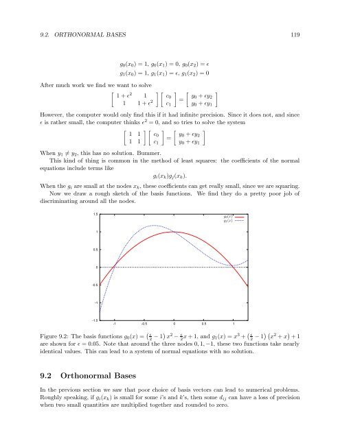
Now we draw a rough sketch of the basis functions. We find they do a pretty poor job of
discriminating around all the nodes.
1.5
g 0 (x)
g 1 (x)
1
0.5
0
-0.5
-1
-1.5
-1 -0.5 0 0.5 1
Figure 9.2: The basis functions g 0 (x) = ( ɛ
2 − 1) x 2 − ɛ 2 x + 1, and g 1(x) = x 3 + ( ɛ
2 − 1) ( x 2 + x ) + 1
are shown for ɛ = 0.05. Note that around the three nodes 0, 1, −1, these two functions take nearly
identical values. This can lead to a system of normal equations with no solution.
9.2 Orthonormal Bases
In the previous section we saw that poor choice of basis vectors can lead to numerical problems.
Roughly speaking, if g i (x k ) is small for some i’s and k’s, then some d ij can have a loss of precision
when two small quantities are multiplied together and rounded to zero.