Numerical Methods Course Notes Version 0.1 (UCSD Math 174, Fall ...

10.2. RUNGE-KUTTA METHODS 131
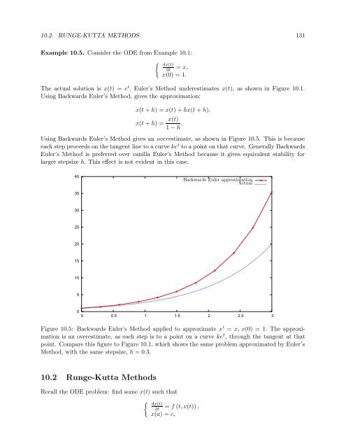
Example 10.5. Consider the ODE from Example 10.1:
{ dx(t)
dt
= x,
x(0) = 1.
The actual solution is x(t) = e t . Euler’s Method underestimates x(t), as shown in Figure 10.1.
Using Backwards Euler’s Method, gives the approximation:
PSfrag replacements
x(t + h) = x(t) + hx(t + h),
x(t + h) = x(t)
1 − h .
Using Backwards Euler’s Method gives an overestimate, as shown in Figure 10.5. This is because
each step proceeds on the tangent line to a curve ke t to a point on that curve. Generally Backwards
Euler’s Method is preferred over vanilla Euler’s Method because it gives equivalent stability for
larger stepsize h. This effect is not evident in this case.
40
Backwards Euler approximation
Actual
35
30
25
20
15
10
5
0
0 0.5 1 1.5 2 2.5 3
Figure 10.5: Backwards Euler’s Method applied to approximate x ′ = x, x(0) = 1. The approximation
is an overestimate, as each step is to a point on a curve ke t , through the tangent at that
point. Compare this figure to Figure 10.1, which shows the same problem approximated by Euler’s
Method, with the same stepsize, h = 0.3.
10.2 Runge-Kutta Methods
Recall the ODE problem: find some x(t) such that
{ dx(t)
dt
= f (t, x(t)) ,
x(a) = c,