Numerical Methods Course Notes Version 0.1 (UCSD Math 174, Fall ...

More documents

Recommendations

Info

$Fractional and operational calculus with generalized fractional ...$

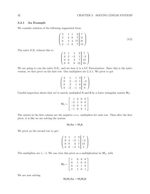
32 CHAPTER 3. SOLVING LINEAR SYSTEMS 3.3.1 An Example We consider solution of the following augmented form: ⎛ ⎜ ⎝ 2 1 1 3 7 4 4 0 7 11 6 5 4 17 31 2 −1 0 7 15 ⎞ ⎟ ⎠ (3.2) The naïve G.E. reduces this to ⎛ ⎜ ⎝ 2 1 1 3 7 0 2 −2 1 −3 0 0 3 7 13 0 0 0 12 18 ⎞ ⎟ ⎠ We are going to run the naïve G.E., and see how it is a LU Factorization. Since this is the naïve version, we first pivot on the first row. Our multipliers are 2, 3, 1. We pivot to get ⎛ ⎜ ⎝ 2 1 1 3 7 0 2 −2 1 −3 0 2 1 8 10 0 −2 −1 4 8 Careful inspection shows that we’ve merely multiplied A and b by a lower triangular matrix M 1 : M 1 = ⎡ ⎢ ⎣ 1 0 0 0 −2 1 0 0 −3 0 1 0 −1 0 0 1 The entries in the first column are the negative e.r.o. multipliers for each row. Thus after the first pivot, it is like we are solving the system M 1 Ax = M 1 b. ⎞ ⎟ ⎠ ⎤ ⎥ ⎦ We pivot on the second row to get: ⎛ ⎜ ⎝ 2 1 1 3 7 0 2 −2 1 −3 0 0 3 7 13 0 0 −3 5 5 ⎞ ⎟ ⎠ The multipliers are 1, −1. We can view this pivot as a multiplication by M 2 , with M 2 = ⎡ ⎢ ⎣ 1 0 0 0 0 1 0 0 0 −1 1 0 0 1 0 1 ⎤ ⎥ ⎦ We are now solving M 2 M 1 Ax = M 2 M 1 b.
3.3. LU FACTORIZATION 33 We pivot on the third row, with a multiplier of −1. Thus we get ⎛ ⎞ 2 1 1 3 7 ⎜ 0 2 −2 1 −3 ⎟ ⎝ 0 0 3 7 13 ⎠ 0 0 0 12 18 We have multiplied by M 3 : We are now solving M 3 = ⎡ ⎢ ⎣ 1 0 0 0 0 1 0 0 0 0 1 0 0 0 1 1 ⎤ ⎥ ⎦ M 3 M 2 M 1 Ax = M 3 M 2 M 1 b. But we have an upper triangular form, that is, if we let ⎡ ⎤ 2 1 1 3 U = ⎢ 0 2 −2 1 ⎥ ⎣ 0 0 3 7 ⎦ 0 0 0 12 Then we have M 3 M 2 M 1 A = U, A = (M 3 M 2 M 1 ) −1 U, A = M 1 −1 M 2 −1 M 3 −1 U, A = LU. We are hoping that L is indeed lower triangular, and has ones on the diagonal. It turns out that the inverse of each M i matrix has a nice form (See Exercise (3.6)). We write them here: ⎡ ⎤ ⎡ ⎤ ⎡ ⎤ 1 0 0 0 1 0 0 0 1 0 0 0 L = ⎢ 2 1 0 0 ⎥ ⎢ 0 1 0 0 ⎥ ⎢ 0 1 0 0 ⎥ ⎣ 3 0 1 0 ⎦ ⎣ 0 1 1 0 ⎦ ⎣ 0 0 1 0 ⎦ 1 0 0 1 0 −1 0 1 0 0 −1 1 = ⎡ ⎢ ⎣ 1 0 0 0 2 1 0 0 3 1 1 0 1 −1 −1 1 ⎤ ⎥ ⎦ This is really crazy: the matrix L looks to be composed of ones on the diagonal and multipliers under the diagonal. Now we check to see if we made any mistakes: LU = = ⎡ ⎢ ⎣ ⎡ ⎢ ⎣ 1 0 0 0 2 1 0 0 3 1 1 0 1 −1 −1 1 2 1 1 3 4 4 0 7 6 5 4 17 2 −1 0 7 ⎤ ⎡ ⎥ ⎢ ⎦ ⎣ ⎤ ⎥ ⎦ = A. 2 1 1 3 0 2 −2 1 0 0 3 7 0 0 0 12 ⎤ ⎥ ⎦
Page 1: Numerical Methods Course Notes Vers
Page 5 and 6: Contents Acknowledgments i 1 Introd
Page 7 and 8: CONTENTS v 8 Integrals and Quadratu
Page 9 and 10: Chapter 1 Introduction 1.1 Taylor
Page 11 and 12: 1.1. TAYLOR’S THEOREM 3 with the
Page 13 and 14: 1.3. EIGENVALUES 5 To correct this
Page 15 and 16: 1.3. EIGENVALUES 7 Example Problem
Page 17 and 18: 1.3. EIGENVALUES 9 for all vectors
Page 19 and 20: Chapter 2 A “Crash” Course in o
Page 21 and 22: 2.1. GETTING STARTED 13 77 22 333 o
Page 23 and 24: 2.2. USEFUL COMMANDS 15 octave:22>
Page 25 and 26: 2.3. PROGRAMMING AND CONTROL 17 x1
Page 27 and 28: 2.4. PLOTTING 19 %just plot Y plot(
Page 29 and 30: 2.4. PLOTTING 21 Exercises (2.1) Wh
Page 31 and 32: Chapter 3 Solving Linear Systems A
Page 33 and 34: 3.1. GAUSSIAN ELIMINATION WITH NAÏ
Page 35 and 36: 3.2. PIVOTING STRATEGIES FOR GAUSSI
Page 37 and 38: 3.2. PIVOTING STRATEGIES FOR GAUSSI
Page 39: 3.3. LU FACTORIZATION 31 appropriat
Page 43 and 44: 3.4. ITERATIVE SOLUTIONS 35 3.3.3 S
Page 45 and 46: 3.4. ITERATIVE SOLUTIONS 37 3.4.2 D
Page 47 and 48: 3.4. ITERATIVE SOLUTIONS 39 We star
Page 49 and 50: 3.4. ITERATIVE SOLUTIONS 41 Now not
Page 51 and 52: 3.4. ITERATIVE SOLUTIONS 43 Remembe
Page 53 and 54: 3.4. ITERATIVE SOLUTIONS 45 is the
Page 55 and 56: Chapter 4 Finding Roots 4.1 Bisecti
Page 57 and 58: 4.2. NEWTON’S METHOD 49 Algorithm
Page 59 and 60: 4.2. NEWTON’S METHOD 51 4.2.2 Pro
Page 61 and 62: 4.3. SECANT METHOD 53 The following
Page 63 and 64: 4.3. SECANT METHOD 55 Since the roo
Page 65 and 66: 4.3. SECANT METHOD 57 relation betw
Page 67 and 68: 4.3. SECANT METHOD 59 (b) f(x) = x
Page 69 and 70: Chapter 5 Interpolation 5.1 Polynom
Page 71 and 72: 5.1. POLYNOMIAL INTERPOLATION 63 2
Page 73 and 74: 5.1. POLYNOMIAL INTERPOLATION 65 Su
Page 75 and 76: 5.2. ERRORS IN POLYNOMIAL INTERPOLA
Page 77 and 78: frag replacements 5.2. ERRORS IN PO
Page 85 and 86: Chapter 6 Spline Interpolation Spli
Page 87 and 88: frag replacements 6.1. FIRST AND SE
Page 89 and 90: 6.2. (NATURAL) CUBIC SPLINES 81 pro
Page 91 and 92:
6.3. B SPLINES 83 The zero degree B
Page 93 and 94:
6.3. B SPLINES 85 Exercises (6.1) I
Page 95 and 96:
Chapter 7 Approximating Derivatives
Page 97 and 98:
7.2. RICHARDSON EXTRAPOLATION 89 7.
Page 99 and 100:
7.2. RICHARDSON EXTRAPOLATION 91 7.
Page 101 and 102:
7.2. RICHARDSON EXTRAPOLATION 93 Ex
Page 103 and 104:
Chapter 8 Integrals and Quadrature
Page 105 and 106:
8.1. THE DEFINITE INTEGRAL 97 Examp
Page 107 and 108:
8.2. TRAPEZOIDAL RULE 99 The compos
Page 109 and 110:
frag replacements 8.2. TRAPEZOIDAL
Page 111 and 112:
8.3. ROMBERG ALGORITHM 103 then def
Page 113 and 114:
8.4. GAUSSIAN QUADRATURE 105 8.4 Ga
Page 115 and 116:
8.4. GAUSSIAN QUADRATURE 107 Exampl
Page 117 and 118:
8.4. GAUSSIAN QUADRATURE 109 Simple
Page 119 and 120:
8.4. GAUSSIAN QUADRATURE 111 Exerci
Page 121 and 122:
8.4. GAUSSIAN QUADRATURE 113 functi
Page 123 and 124:
Chapter 9 Least Squares 9.1 Least S
Page 125 and 126:
9.1. LEAST SQUARES 117 The answer i
Page 127 and 128:
9.2. ORTHONORMAL BASES 119 g 0 (x 0
Page 129 and 130:
frag replacements 9.2. ORTHONORMAL
Page 131 and 132:
Chapter 10 Ordinary Differential Eq
Page 133 and 134:
10.1. ELEMENTARY METHODS 125 value
Page 135 and 136:
frag replacements 10.1. ELEMENTARY
Page 137 and 138:
10.1. ELEMENTARY METHODS 129 It tur
Page 139 and 140:
10.2. RUNGE-KUTTA METHODS 131 Examp
Page 141 and 142:
10.2. RUNGE-KUTTA METHODS 133 We no
Page 143 and 144:
10.3. SYSTEMS OF ODES 135 Example 1
Page 145 and 146:
10.3. SYSTEMS OF ODES 137 Euler’s
Page 147 and 148:
10.3. SYSTEMS OF ODES 139 have to b
Page 149 and 150:
10.3. SYSTEMS OF ODES 141 4.5 4 3.5
Page 151 and 152:
10.3. SYSTEMS OF ODES 143 (10.9) Im
Page 153 and 154:
Appendix A Old Exams A.1 First Midt
Page 155 and 156:
A.3. FINAL EXAM, FALL 2003 147 •
Page 157 and 158:
A.4. FIRST MIDTERM, FALL 2004 149
Page 159 and 160:
A.5. SECOND MIDTERM, FALL 2004 151
Page 161 and 162:
A.6. FINAL EXAM, FALL 2004 153 P5 (
Page 163 and 164:
Appendix B GNU Free Documentation L
Page 165 and 166:
157 F. Include, immediately after t
Page 167 and 168:
Bibliography [1] Guillaume Bal. Lec
show all

Numerical Methods Course Notes Version 0.1 (UCSD Math 174, Fall ...

Create successful ePaper yourself

Delete template?

Save as template?