Numerical Methods Course Notes Version 0.1 (UCSD Math 174, Fall ...

More documents

Recommendations

Info

$Fractional and operational calculus with generalized fractional ...$

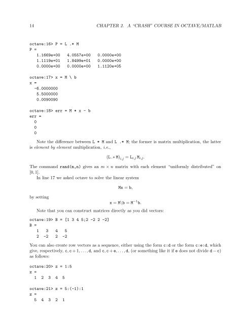
14 CHAPTER 2. A “CRASH” COURSE IN OCTAVE/MATLAB octave:16> P = L .* M P = 1.1669e+00 4.0557e+00 0.0000e+00 1.1119e+01 1.8499e+01 0.0000e+00 0.0000e+00 0.0000e+00 1.1120e+05 octave:17> x = M \ b x = -6.0000000 5.5000000 0.0090090 octave:18> err = M * x - b err = 0 0 0 Note the difference between L * M and L .* M; the former is matrix multiplication, the latter is element by element multiplication, i.e., (L .∗ M) i,j = L i,j M i,j . The command rand(m,n) gives an m × n matrix with each element “uniformly distributed” on [0, 1]. In line 17 we asked octave to solve the linear system by setting Mx = b, x = M\b = M −1 b. Note that you can construct matrices directly as you did vectors: octave:19> B = [1 3 4 5;2 -2 2 -2] B = 1 3 4 5 2 -2 2 -2 You can also create row vectors as a sequence, either using the form c:d or the form c:e:d, which give, respectively, c, c + 1, . . . , d, and c, c + e, . . . , d, (or something like it if e does not divide d − c) as follows: octave:20> z = 1:5 z = 1 2 3 4 5 octave:21> z = 5:(-1):1 z = 5 4 3 2 1
2.2. USEFUL COMMANDS 15 octave:22> z = 5:(-2):1 z = 5 3 1 octave:23> z = 2:3:11 z = 2 5 8 11 octave:24> z = 2:3:10 z = 2 5 8 2.2 Useful Commands Here’s a none too complete listing of useful commands in octave: • help is the most useful command. • floor(X) returns the largest integer not greater than X. If X is a vector or matrix, it computes the floor element-wise. This behavior is common in octave: many functions which we normally think of as applicable to scalars can be applied to matrices, with the result computed elementwise. • ceil(X) returns the smallest integer not less than X, computed element-wise. • sin(X), cos(X), tan(X), atan(X), sqrt(X), returns the sine, cosine, tangent, arctangent, square root of X, computed elementwise. • exp(X) returns e X , elementwise. • abs(X) returns |X| , elementwise. • norm(X) returns the norm of X; if X is a vector, this is the L 2 norm: ‖X‖ 2 = ( ∑ i X 2 i ) 1/2 , if X is a matrix, it is the matrix norm subordinate to the L 2 norm. You can compute other norms with norm(X,p) where p is a number, to get the L p norm, or with p one of Inf, -Inf, etc. • zeros(m,n) returns an m × n matrix of all zeros. • eye(m) returns the m × m identity matrix. • [m,n] = size(A) returns the number of rows, columns of A. • length(v) returns the length of vector v, or the larger dimension if v is a matrix. • diag(v) returns the diagonal matrix with vector v as diagonal. diag(M) returns as a vector, the diagonal of matrix v. Thus diag(diag(v)) is v for vector v, but diag(diag(M)) is the diagonal part of matrix M. • toeplitz(v) returns the Toeplitz matrix associated with vector v. That is ⎡ toeplitz(v) = ⎢ ⎣ v(1) v(2) v(3) · · · v(n) v(2) v(1) v(2) · · · v(n − 1) v(3) v(2) v(1) · · · v(n − 2) . . . . .. . v(n) v(n − 1) v(n − 2) · · · v(1) ⎤ ⎥ ⎦
Page 1: Numerical Methods Course Notes Vers
Page 5 and 6: Contents Acknowledgments i 1 Introd
Page 7 and 8: CONTENTS v 8 Integrals and Quadratu
Page 9 and 10: Chapter 1 Introduction 1.1 Taylor
Page 11 and 12: 1.1. TAYLOR’S THEOREM 3 with the
Page 13 and 14: 1.3. EIGENVALUES 5 To correct this
Page 15 and 16: 1.3. EIGENVALUES 7 Example Problem
Page 17 and 18: 1.3. EIGENVALUES 9 for all vectors
Page 19 and 20: Chapter 2 A “Crash” Course in o
Page 21: 2.1. GETTING STARTED 13 77 22 333 o
Page 25 and 26: 2.3. PROGRAMMING AND CONTROL 17 x1
Page 27 and 28: 2.4. PLOTTING 19 %just plot Y plot(
Page 29 and 30: 2.4. PLOTTING 21 Exercises (2.1) Wh
Page 31 and 32: Chapter 3 Solving Linear Systems A
Page 33 and 34: 3.1. GAUSSIAN ELIMINATION WITH NAÏ
Page 35 and 36: 3.2. PIVOTING STRATEGIES FOR GAUSSI
Page 37 and 38: 3.2. PIVOTING STRATEGIES FOR GAUSSI
Page 39 and 40: 3.3. LU FACTORIZATION 31 appropriat
Page 41 and 42: 3.3. LU FACTORIZATION 33 We pivot o
Page 43 and 44: 3.4. ITERATIVE SOLUTIONS 35 3.3.3 S
Page 45 and 46: 3.4. ITERATIVE SOLUTIONS 37 3.4.2 D
Page 47 and 48: 3.4. ITERATIVE SOLUTIONS 39 We star
Page 49 and 50: 3.4. ITERATIVE SOLUTIONS 41 Now not
Page 51 and 52: 3.4. ITERATIVE SOLUTIONS 43 Remembe
Page 53 and 54: 3.4. ITERATIVE SOLUTIONS 45 is the
Page 55 and 56: Chapter 4 Finding Roots 4.1 Bisecti
Page 57 and 58: 4.2. NEWTON’S METHOD 49 Algorithm
Page 59 and 60: 4.2. NEWTON’S METHOD 51 4.2.2 Pro
Page 61 and 62: 4.3. SECANT METHOD 53 The following
Page 63 and 64: 4.3. SECANT METHOD 55 Since the roo
Page 65 and 66: 4.3. SECANT METHOD 57 relation betw
Page 67 and 68: 4.3. SECANT METHOD 59 (b) f(x) = x
Page 69 and 70: Chapter 5 Interpolation 5.1 Polynom
Page 71 and 72: 5.1. POLYNOMIAL INTERPOLATION 63 2
Page 73 and 74:
5.1. POLYNOMIAL INTERPOLATION 65 Su
Page 75 and 76:
5.2. ERRORS IN POLYNOMIAL INTERPOLA
Page 77 and 78:
frag replacements 5.2. ERRORS IN PO
Page 79 and 80:
Page 81 and 82:
Page 83 and 84:
Page 85 and 86:
Chapter 6 Spline Interpolation Spli
Page 87 and 88:
frag replacements 6.1. FIRST AND SE
Page 89 and 90:
6.2. (NATURAL) CUBIC SPLINES 81 pro
Page 91 and 92:
6.3. B SPLINES 83 The zero degree B
Page 93 and 94:
6.3. B SPLINES 85 Exercises (6.1) I
Page 95 and 96:
Chapter 7 Approximating Derivatives
Page 97 and 98:
7.2. RICHARDSON EXTRAPOLATION 89 7.
Page 99 and 100:
7.2. RICHARDSON EXTRAPOLATION 91 7.
Page 101 and 102:
7.2. RICHARDSON EXTRAPOLATION 93 Ex
Page 103 and 104:
Chapter 8 Integrals and Quadrature
Page 105 and 106:
8.1. THE DEFINITE INTEGRAL 97 Examp
Page 107 and 108:
8.2. TRAPEZOIDAL RULE 99 The compos
Page 109 and 110:
frag replacements 8.2. TRAPEZOIDAL
Page 111 and 112:
8.3. ROMBERG ALGORITHM 103 then def
Page 113 and 114:
8.4. GAUSSIAN QUADRATURE 105 8.4 Ga
Page 115 and 116:
8.4. GAUSSIAN QUADRATURE 107 Exampl
Page 117 and 118:
8.4. GAUSSIAN QUADRATURE 109 Simple
Page 119 and 120:
8.4. GAUSSIAN QUADRATURE 111 Exerci
Page 121 and 122:
8.4. GAUSSIAN QUADRATURE 113 functi
Page 123 and 124:
Chapter 9 Least Squares 9.1 Least S
Page 125 and 126:
9.1. LEAST SQUARES 117 The answer i
Page 127 and 128:
9.2. ORTHONORMAL BASES 119 g 0 (x 0
Page 129 and 130:
frag replacements 9.2. ORTHONORMAL
Page 131 and 132:
Chapter 10 Ordinary Differential Eq
Page 133 and 134:
10.1. ELEMENTARY METHODS 125 value
Page 135 and 136:
frag replacements 10.1. ELEMENTARY
Page 137 and 138:
10.1. ELEMENTARY METHODS 129 It tur
Page 139 and 140:
10.2. RUNGE-KUTTA METHODS 131 Examp
Page 141 and 142:
10.2. RUNGE-KUTTA METHODS 133 We no
Page 143 and 144:
10.3. SYSTEMS OF ODES 135 Example 1
Page 145 and 146:
10.3. SYSTEMS OF ODES 137 Euler’s
Page 147 and 148:
10.3. SYSTEMS OF ODES 139 have to b
Page 149 and 150:
10.3. SYSTEMS OF ODES 141 4.5 4 3.5
Page 151 and 152:
10.3. SYSTEMS OF ODES 143 (10.9) Im
Page 153 and 154:
Appendix A Old Exams A.1 First Midt
Page 155 and 156:
A.3. FINAL EXAM, FALL 2003 147 •
Page 157 and 158:
A.4. FIRST MIDTERM, FALL 2004 149
Page 159 and 160:
A.5. SECOND MIDTERM, FALL 2004 151
Page 161 and 162:
A.6. FINAL EXAM, FALL 2004 153 P5 (
Page 163 and 164:
Appendix B GNU Free Documentation L
Page 165 and 166:
157 F. Include, immediately after t
Page 167 and 168:
Bibliography [1] Guillaume Bal. Lec
show all

Numerical Methods Course Notes Version 0.1 (UCSD Math 174, Fall ...

You also want an ePaper? Increase the reach of your titles

Delete template?

Save as template?