Numerical Methods Course Notes Version 0.1 (UCSD Math 174, Fall ...

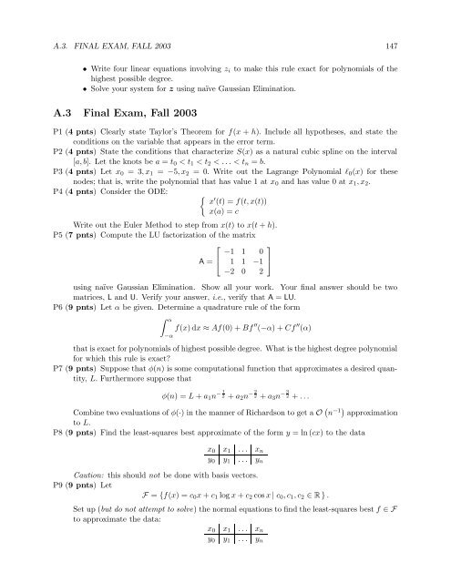
A.3. FINAL EXAM, FALL 2003 147
• Write four linear equations involving z i to make this rule exact for polynomials of the
highest possible degree.
• Solve your system for z using naïve Gaussian Elimination.
A.3 Final Exam, Fall 2003
P1 (4 pnts) Clearly state Taylor’s Theorem for f(x + h). Include all hypotheses, and state the
conditions on the variable that appears in the error term.
P2 (4 pnts) State the conditions that characterize S(x) as a natural cubic spline on the interval
[a, b]. Let the knots be a = t 0 < t 1 < t 2 < . . . < t n = b.
P3 (4 pnts) Let x 0 = 3, x 1 = −5, x 2 = 0. Write out the Lagrange Polynomial l 0 (x) for these
nodes; that is, write the polynomial that has value 1 at x 0 and has value 0 at x 1 , x 2 .
P4 (4 pnts) Consider the ODE:
{ x ′ (t) = f(t, x(t))
x(a) = c
Write out the Euler Method to step from x(t) to x(t + h).
P5 (7 pnts) Compute the LU factorization of the matrix
⎡
−1 1
⎤
0
A = ⎣ 1 1 −1 ⎦
−2 0 2
using naïve Gaussian Elimination. Show all your work. Your final answer should be two
matrices, L and U. Verify your answer, i.e., verify that A = LU.
P6 (9 pnts) Let α be given. Determine a quadrature rule of the form
∫ α
−α
f(x) dx ≈ Af(0) + Bf ′′ (−α) + Cf ′′ (α)
that is exact for polynomials of highest possible degree. What is the highest degree polynomial
for which this rule is exact?
P7 (9 pnts) Suppose that φ(n) is some computational function that approximates a desired quantity,
L. Furthermore suppose that
φ(n) = L + a 1 n − 1 2 + a 2 n − 2 2 + a 3 n − 3 2 + . . .
Combine two evaluations of φ(·) in the manner of Richardson to get a O ( n −1) approximation
to L.
P8 (9 pnts) Find the least-squares best approximate of the form y = ln (cx) to the data
x 0 x 1 . . . x n
y 0 y 1 . . . y n
Caution: this should not be done with basis vectors.
P9 (9 pnts) Let
F = {f(x) = c 0 x + c 1 log x + c 2 cos x | c 0 , c 1 , c 2 ∈ R } .
Set up (but do not attempt to solve) the normal equations to find the least-squares best f ∈ F
to approximate the data:
x 0 x 1 . . . x n
y 0 y 1 . . . y n