Numerical Methods Course Notes Version 0.1 (UCSD Math 174, Fall ...

3.4. ITERATIVE SOLUTIONS 35
3.3.3 Some Theory
We aren’t doing much proving here. The following theorem has an ugly proof in the Cheney &
Kincaid [7].
Theorem 3.3. If A is an n × n matrix, and naïve Gaussian Elimination does not encounter a zero
pivot, then the algorithm generates a LU factorization of A, where L is the lower triangular part of
the output matrix, and U is the upper triangular part.
This theorem relies on us using the fancy version of G.E., which saves the multipliers in the
spots where there should be zeros. If correctly implemented, then, L is the lower triangular part
but with ones put on the diagonal.
This theorem is proved in Cheney & Kincaid [7]. This appears to me to be a case of something
which can be better illustrated with an example or two and some informal investigation. The proof
is an unillustrating index-chase–read it at your own risk.
3.3.4 Computing Inverses
We consider finding the inverse of A. Since
AA −1 = I,
then the j th column of the inverse A −1 solves the equation
Ax = e j ,
where e j is the column matrix of all zeros, but with a one in the j th position.
Thus we can find the inverse of A by running n linear solves. Obviously we are only going
to run G.E. once, to put the matrix in LU form, then run n solves using forward and backward
substitutions.
3.4 Iterative Solutions
Recall we are trying to solve
Ax = b.
We examine the computational cost of Gaussian Elimination to motivate the search for an alternative
algorithm.
3.4.1 An Operation Count for Gaussian Elimination
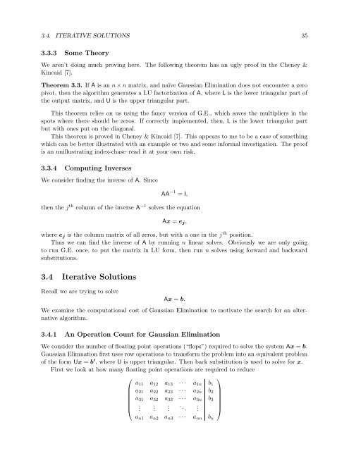
We consider the number of floating point operations (“flops”) required to solve the system Ax = b.
Gaussian Elimnation first uses row operations to transform the problem into an equivalent problem
of the form Ux = b ′ , where U is upper triangular. Then back substitution is used to solve for x.
First we look at how many floating point operations are required to reduce
⎛
⎞
a 11 a 12 a 13 · · · a 1n b 1
a 21 a 22 a 23 · · · a 2n b 2
a 31 a 32 a 33 · · · a 3n b 3
⎜
⎝
.
. . . ..
⎟
. ⎠
a n1 a n2 a n3 · · · a nn b n