- Page 1 and 2:
Nuclear Development ACTINIDE AND FI
- Page 3 and 4:
FOREWORD The objective of the OECD/
- Page 5 and 6:
TABLE OF CONTENTS Foreword ........
- Page 7 and 8:
EXECUTIVE SUMMARY More than 160 par
- Page 9:
identified. In the fuel area, labor
- Page 12 and 13:
17:20-19:05 Session III: Partitioni
- Page 14 and 15:
Poster sessions Poster session: Par
- Page 17 and 18:
WELCOME ADDRESS Lucila Izquierdo Ge
- Page 19 and 20:
WELCOME ADDRESS Michel Hugon Co-ord
- Page 21 and 22:
WELCOME ADDRESS Philippe Savelli De
- Page 23:
developments. This will surely beco
- Page 26 and 27:
use of FBRs for transmutation toget
- Page 28 and 29:
view, i.e. better use of uranium an
- Page 30 and 31:
W. Forsberg proposes to reduce the
- Page 32 and 33:
1. From the open fuel cycle to the
- Page 34 and 35:
Figures 2 and 3 show the radiotoxic
- Page 36 and 37:
Denoting the transuranic (TRU) or m
- Page 38 and 39:
or, in terms of the fuel burn-up an
- Page 40 and 41:
quantities of LWR-MOX and FR-MOX wi
- Page 42 and 43:
view of the historic development, t
- Page 44 and 45:
Table 5. Assumptions for transmutat
- Page 46 and 47:
separating troublesome fission prod
- Page 48 and 49:
REFERENCES [1] L.H. Baetslé, Ch. D
- Page 51 and 52:
SESSION III Partitioning Chairs: J.
- Page 53 and 54:
OVERVIEW OF THE HYDROMETALLURGICAL
- Page 55 and 56:
2.1.3 Consequences Owing to the fac
- Page 57 and 58:
The extraction and separation mecha
- Page 59 and 60:
extractant was observed. As a conse
- Page 61 and 62:
2.3.2 Examples of strategies and
- Page 63 and 64:
3. Conclusions and perspectives 3.1
- Page 65 and 66:
SESSION IV Basic Physics, Materials
- Page 67 and 68:
TRANSMUTATION: A DECADE OF REVIVAL
- Page 69 and 70:
2.1 The IFR concept and the homogen
- Page 71 and 72:
2.3 Dedicated systems Making again
- Page 73 and 74:
compound “macro-dispersed” in M
- Page 75 and 76:
Figure 3. Sketch of ADS, liquid met
- Page 77 and 78:
3.3.2.1 The MEGAPIE project [40] ME
- Page 79 and 80:
3.3.2.2 The MUSE experiments The MU
- Page 81 and 82:
Figure 8. Comparison of the neutron
- Page 83 and 84:
Figure 9. Scenarios at equilibrium
- Page 85 and 86:
goals in this field. Since once-thr
- Page 87 and 88:
• The use of Thorium in PWRs alwa
- Page 89 and 90:
• Understanding of the role of AD
- Page 91 and 92:
[17] Y. Arai, T. Ogawa, Research on
- Page 93:
SESSION V Transmutation Systems and
- Page 96 and 97:
1. Introduction The term ADS compre
- Page 98 and 99:
• Safety should be “designed in
- Page 100 and 101:
3. Minor actinide and/or transurani
- Page 102 and 103:
Table 2. Values of Dj (neutron cons
- Page 104 and 105:
Table 4. Delayed neutron fraction I
- Page 106 and 107:
Figure 4. η (Neutrons released per
- Page 108 and 109:
Table 5. ADS Distinguishing feature
- Page 110 and 111:
While a favourable ADS safety featu
- Page 112 and 113:
Optimised mixes of MA and Pu can be
- Page 114 and 115:
Moreover, the fuel is where neutron
- Page 116 and 117:
REFERENCES [1] L. Van den Durpel et
- Page 118 and 119:
[19] D.C. Wade and E. Fujita, Trend
- Page 121 and 122:
POSTER SESSION Basic Physics: Nucle
- Page 123:
To conclude, this poster session in
- Page 126 and 127:
Five other papers related to ADS co
- Page 129:
SESSION I OVERVIEW OF NATIONAL AND
- Page 132 and 133:
1. Current activities for radioacti
- Page 134 and 135:
3.2 Results to date and analyses of
- Page 136 and 137:
3.2.5.2 JNC JNC is considering the
- Page 138 and 139:
4.6 Short-term increase in radiatio
- Page 140 and 141:
Annex 1 R&D scheme for partitioning
- Page 142 and 143:
Annex 3 Members of the Advisory Com
- Page 144 and 145:
plutonium can be recycled in pressu
- Page 146 and 147:
choices and the implementation of m
- Page 148 and 149:
1. Introduction Since the 5th Infor
- Page 150 and 151:
strata” approach which would invo
- Page 153 and 154:
IAEA ACTIVITIES IN THE AREA OF EMER
- Page 155 and 156:
actually started to do so) because
- Page 157 and 158:
establishment of an international R
- Page 159 and 160:
The accelerator driven transmutatio
- Page 161 and 162:
substantiate this recommendation, s
- Page 163 and 164:
current, advanced and innovative nu
- Page 165 and 166:
ACCELERATOR DRIVEN SUB-CRITICAL SYS
- Page 167 and 168:
demonstration of feasibility of a E
- Page 169 and 170:
An extended “skeleton” for ADS
- Page 171 and 172:
• Fertile support (uranium) is no
- Page 173:
7. Conclusions The TWG under the ch
- Page 176 and 177:
1. Introduction The priorities for
- Page 178 and 179:
In the EURATOM Fourth Framework Pro
- Page 180 and 181:
Table 2. Cluster on transmutation-t
- Page 182 and 183:
6. Community research for the perio
- Page 184 and 185:
REFERENCES [1] “Council Decision
- Page 186 and 187:
1. Introduction Back in 1989, the O
- Page 188 and 189:
would need the continuation of tech
- Page 190 and 191:
individual isotopes as a function o
- Page 192 and 193:
Therefore, while there is continuin
- Page 194 and 195:
[9] OECD/NEA, Overview of Physics A
- Page 197 and 198:
RECENT TOPICS IN R&D FOR THE OMEGA
- Page 199 and 200:
Figure 1. Partitioning and transmut
- Page 201 and 202:
The present 4-GPP necessitates a pr
- Page 203 and 204:
5. Concluding remarks In 1999, the
- Page 205:
REFERENCES [1] T. Mukaiyama, T. Tak
- Page 208 and 209:
1. Introduction CIEMAT is actively
- Page 210 and 211:
adiotoxicity to be managed could al
- Page 212 and 213:
Figure 3. Mass composition of the d
- Page 214 and 215:
Figure 6. Fuel cycle assumed in the
- Page 216 and 217:
the 4 batches scheme, allowing to a
- Page 218 and 219:
Figure 11. Transmutation efficiency
- Page 220 and 221:
1. Introduction Spent fuels of mode
- Page 222 and 223:
Figure 3. A change in radiotoxicity
- Page 224 and 225:
These dependencies are shown on Fig
- Page 226 and 227:
When increasing the moderator fract
- Page 228 and 229:
Even greater power increases are ob
- Page 230 and 231:
The effect of a moderator volume fr
- Page 232 and 233:
Table 11. Different isotopes contri
- Page 234 and 235:
Thus the transmutation of such FPs
- Page 237 and 238:
ASSESSMENT OF NUCLEAR POWER SCENARI
- Page 239 and 240:
elease probabilities. The time dist
- Page 241 and 242:
Table 2. Annual heavy nuclide contr
- Page 243 and 244:
Figure 3. Reduction of potential ra
- Page 245 and 246:
DISPOSAL OF PARTITIONING-TRANSMUTAT
- Page 247 and 248:
Figure 2. Decay heat from SNF 2000
- Page 249 and 250:
Figure 3. Shorter-lived HHR reposit
- Page 251 and 252:
4. Management of low-heat, long-liv
- Page 253 and 254:
isotope from other caesium isotopes
- Page 255 and 256:
THE AMSTER CONCEPT J. Vergnes 1 , D
- Page 257 and 258:
Figure 1. Layout diagram of the mol
- Page 259 and 260:
Table 1. Definition of configuratio
- Page 261 and 262:
We therefore adopted a partial purg
- Page 263 and 264:
conceivable. Thus by increasing the
- Page 265 and 266:
6. R&D needed to validate the AMSTE
- Page 267:
SESSION III PARTITIONING J.P. Glatz
- Page 271 and 272:
PARTITIONING-SEPARATION OF METAL IO
- Page 273 and 274:
The terpyridyl reagent (ligand L 1
- Page 275 and 276:
Figure 2. The synthesis of ADTPTZ a
- Page 277 and 278:
2.4 Implications for partitioning T
- Page 279 and 280:
SEPARATION OF MINOR ACTINIDES FROM
- Page 281 and 282:
installed in a hot cell. The feed w
- Page 283 and 284:
the concentrations of U, Pu and Np
- Page 285 and 286:
Table 2 shows the recovery in the r
- Page 287 and 288:
PARTITIONING ANIONIC AGENTS BASED O
- Page 289 and 290:
which of these, the Co 3+ , Fe 3+ a
- Page 291 and 292:
This dianionic species must be extr
- Page 293 and 294:
Figure 6 Ph 2 P acetone PPh 2 H2 O
- Page 295 and 296:
Figure 9 H 3 C RO(CH 2 )n CH 3 (CH
- Page 297:
[7] J. Rais and P. Selucky, Nucleon
- Page 301 and 302:
PYROCHEMICAL PROCESSING OF IRRADIAT
- Page 303 and 304:
The metallic cadmium product of the
- Page 305 and 306:
Figure 2. Schematic flow-sheet for
- Page 307 and 308:
R&D OF PYROCHEMICAL PARTITIONING IN
- Page 309 and 310:
(first of all pumps) for fluoride m
- Page 311 and 312:
4. Research on material and equipme
- Page 313:
REFERENCES [1] Uhlir J., Pyrochemic
- Page 316 and 317:
1. Introduction The increasing inte
- Page 318 and 319:
Figure 2. Stainless steel box with
- Page 320 and 321:
Figure 4. U deposit on solid cathod
- Page 322 and 323:
Figure 7. Schematic flow of the cou
- Page 324 and 325:
actinide elements from spent (metal
- Page 327 and 328:
DEVELOPMENT OF PLUTONIUM RECOVERY P
- Page 329 and 330:
uranium dendrite and that uranium c
- Page 331 and 332:
Table 1. Conditions and results of
- Page 333 and 334:
Cathode potential went down to -1.6
- Page 335 and 336:
Figure 6. Change of LCC potential i
- Page 337 and 338:
Figure 9. Relation between Pu conce
- Page 339 and 340:
consideration described in the prec
- Page 341:
[13] Y. Arai, S. Fukushima, K. Shio
- Page 345:
SESSION IV BASIC PHYSICS, MATERIALS
- Page 348 and 349:
1. Introduction The reduction of th
- Page 350 and 351:
agrees ours within limits of errors
- Page 352 and 353:
Figure 1. Thermal neutron capture c
- Page 354 and 355:
[18] A.P. Baerg, R.M. Bartholomew,
- Page 356 and 357:
1. Introduction Nowadays it is well
- Page 358 and 359:
In order to describe the inter-nucl
- Page 360 and 361:
kind of measurements allow to chara
- Page 362 and 363:
Figure 6. Two-dimensional cluster p
- Page 364 and 365:
Figure 8. Excitation functions for
- Page 366 and 367:
REFERENCES [1] D. Ridikas, thesis,
- Page 368 and 369:
1. Introduction Since 1991, the Com
- Page 370 and 371:
Experimental reactivity control tec
- Page 372 and 373:
Table 2. Neutron intensities Target
- Page 374 and 375:
experimental channels (horizontal a
- Page 376 and 377:
376
- Page 378 and 379:
Table 3. Planned experimental progr
- Page 380 and 381:
1. Introduction and benchmark speci
- Page 382 and 383:
neutrons. Since the neutron flux is
- Page 384 and 385:
Figure 2. Microscopic capture cross
- Page 386 and 387:
Figure 4. k eff variation in the st
- Page 388 and 389:
2.4 Neutron flux distribution One r
- Page 390 and 391:
etween the highest and the lowest v
- Page 392 and 393:
The isotope specific β eff values
- Page 395:
SESSION IV BASIC PHYSICS, MATERIALS
- Page 398 and 399:
1. Introduction Due to its excellen
- Page 400 and 401:
Figure 2. Tests scheme 0 340 h. 1 0
- Page 402 and 403:
Figure 4. Auger depth profile conce
- Page 404 and 405:
Figure 8. Auger depth profile conce
- Page 406 and 407:
deposited at the cold zone, and the
- Page 408 and 409:
inner layer grows inward from the o
- Page 410 and 411:
[8] V.M. Fedirko, O.I. Eliseeva, V.
- Page 412 and 413:
1. Introduction One of the main par
- Page 414 and 415:
3. Tantalum target irradiation The
- Page 416 and 417:
At 10-MeV neutron irradiation, radi
- Page 418 and 419:
1. Introduction HYPER (HYbrid Power
- Page 420 and 421:
this study, we used an orthogonal c
- Page 422 and 423:
Figure 5. Temperature distribution
- Page 424 and 425:
Figure 7. Thermal stress distributi
- Page 427 and 428:
FUEL/TARGET CONCEPTS FOR TRANSMUTAT
- Page 429 and 430:
(U 0.55 Pu 0.4 Np 0.05 )O 2 fuels w
- Page 431 and 432:
Figure 3. Left: Ceramograph of a (Z
- Page 433 and 434:
Figure 6. Left: ceramograph of a(Zr
- Page 435 and 436:
AMERICIUM TARGETS IN FAST REACTORS
- Page 437 and 438:
The reference case for all comparis
- Page 439 and 440:
It should be underlined that this c
- Page 441 and 442:
Cases Table 3. Heterogeneous recycl
- Page 443 and 444:
• A later step could be to add Cm
- Page 445 and 446:
RESEARCH ON NITRIDE FUEL AND PYROCH
- Page 447 and 448:
temperature for (Cm,Pu)N followed t
- Page 449 and 450:
Figure 1. Temperature dependence of
- Page 451 and 452:
The difference of two fuel pins exi
- Page 453 and 454:
In addition to the voltammetric stu
- Page 455 and 456:
2 wt% of Pu at 773 K. For the momen
- Page 457:
[13] M. Akabori, M. Takano, A. Itoh
- Page 460 and 461:
1. Introduction For the management
- Page 462 and 463:
The scientific feasibility of pluto
- Page 464 and 465:
Another option using a basis of sta
- Page 466 and 467:
6.2.1 Inert matrices 6.2.1.1 MgAl 2
- Page 468 and 469:
eached respectively 38.5% and 70% F
- Page 470 and 471:
Figure 4. Experiments for MA transm
- Page 472 and 473:
Figure 5a. Ecrix B rig Figure 5b. E
- Page 474 and 475:
A CEA/Minatom work programme is und
- Page 476 and 477:
9.3 Programme for dedicated fuels F
- Page 478 and 479:
[14] R.J.M. Konings et al., The EFT
- Page 480 and 481:
1. Introduction An accelerator driv
- Page 482 and 483:
corresponding Pb-Bi velocity is 1.1
- Page 484 and 485:
the fission product target. The rod
- Page 486 and 487:
fuel rods are at the TRU assembly t
- Page 489:
SESSION V TRANSMUTATION SYSTEMS AND
- Page 492 and 493:
1. Introduction Since the 50s, nitr
- Page 494 and 495:
A three dimensional model of a sub-
- Page 496 and 497:
Figure 4. Change in k-eigenvalue fo
- Page 498 and 499:
[4] Y. Arai et al., Experimental Re
- Page 500 and 501:
Nomenclature ADS: ATW: GT-MHR: LOF:
- Page 502 and 503:
Regarding switching off the beam, o
- Page 504 and 505:
Figure 3. Beam blocking 10 min (200
- Page 506 and 507:
Figure 7. A possible scenario for n
- Page 508 and 509:
[15] Greenspan E. et al., The Encap
- Page 510 and 511:
1. Introduction In the EADF design
- Page 512 and 513:
Equation (6) can be improved by con
- Page 514 and 515:
where L is obtained by a summation
- Page 516 and 517:
Figure 1. The natural convection im
- Page 518 and 519:
Figure 4 shows the temperature tren
- Page 520 and 521:
[12] P.H. Wakker, Thermal Hydraulic
- Page 522 and 523:
1. Introduction Research and develo
- Page 524 and 525:
Table 2. Core design parameters for
- Page 526 and 527:
2.2 Representation of MA transmutat
- Page 528 and 529:
Figure 1(b) shows the cases for the
- Page 530 and 531:
It is found that the higher MA tran
- Page 532 and 533:
REFERENCES [1] T. Ikegami, H. Hayas
- Page 534 and 535:
1. Introduction The management of t
- Page 536 and 537:
Table 1. Core performance of MA and
- Page 538 and 539:
Figure 3. Nuclear electricity capac
- Page 540 and 541:
Table 3. Experimental items at PEF
- Page 542 and 543:
REFERENCES [1] Takano H., Akie H.,
- Page 544 and 545:
1. Introduction and background The
- Page 546 and 547:
neutron source, the reactor can mai
- Page 548 and 549:
atoms. For fuel region Rf = 2.5 cm,
- Page 550 and 551:
Figure 3. Neutron flux spectra for
- Page 552 and 553:
A possible way to maintain the k ef
- Page 554 and 555:
higher than 99% of 239 Pu, and high
- Page 557 and 558:
TRANSMUTATION OF NUCLEAR WASTES WIT
- Page 559 and 560:
Figure 1. PBT conceptual view Table
- Page 561 and 562:
very tight holders for fission frag
- Page 563 and 564:
5. Cooling system A preliminary des
- Page 565 and 566:
spectral densities [10,11] and can
- Page 567 and 568:
MYRRHA, A MULTI-PURPOSE ADS FOR R&D
- Page 569 and 570:
hexagonal assemblies of 122 mm plat
- Page 571 and 572:
to achieve the requested performanc
- Page 573 and 574:
3 MYRRHA associated R&D programme F
- Page 575 and 576:
collaboration with Forschungszentru
- Page 577:
• Industrial partners, in particu
- Page 580 and 581:
1. Introduction The transmutation o
- Page 582 and 583:
Existing accelerators have been des
- Page 584 and 585:
suggested to look for an innovative
- Page 586 and 587:
Table 1. Main lead-bismuth eutectic
- Page 588 and 589:
4.3 The core The basic fuel sub-ass
- Page 590 and 591:
Figure 1. Experimental accelerator
- Page 593 and 594:
HELIUM-COOLED REACTOR TECHNOLOGIES
- Page 595 and 596:
of its potential use in nuclear wea
- Page 597 and 598:
Figure 2. Neutron flux distribution
- Page 599 and 600:
atio. Given this rate of destructio
- Page 601 and 602:
Figure 5. Irradiated TRISO particle
- Page 603 and 604:
in ceramic-coated microspheres of t
- Page 605 and 606:
(LOCA) event. The effect on this fe
- Page 607 and 608:
Figure 13. Elevation AD-FMHR The fa
- Page 609:
Deep burn-up of 239 Pu and fissiona
- Page 613:
POSTER SESSION PARTITIONING M.J. Hu
- Page 616 and 617:
1. Introduction The study of the be
- Page 618 and 619:
Plutonium was simulated with the no
- Page 620 and 621:
The influence of uranium and pluton
- Page 622 and 623:
The influence of uranium and pluton
- Page 624 and 625:
REFERENCES [1] I.I. Nazarenko, A.M.
- Page 626 and 627:
1. Introduction The long-term radio
- Page 628 and 629:
Ce Ce 3+ Cl - Cl 2 The voltammogram
- Page 630 and 631:
Figure 3. Chronopotentiograms for t
- Page 632 and 633:
Figure 4. Potentiometric titrations
- Page 634 and 635:
Experimental solubilization tests w
- Page 636 and 637:
[13] H. Flood T. Förland and K. Mo
- Page 638 and 639:
1. Introduction The separation of l
- Page 640 and 641:
Figure 4. Synthesis of amides 11-15
- Page 642 and 643:
1. Introduction Over the recent yea
- Page 644 and 645:
2.3.2 Set-up We set up a single HFM
- Page 646 and 647:
lower flow rates, Am(III) would be
- Page 649 and 650:
THE POTENTIAL OF NANO- AND MICROPAR
- Page 651 and 652:
efficiently and stable. This can be
- Page 653 and 654:
Figure 1a. Zetapotential of NTA-mod
- Page 655 and 656:
Scheme 7. Magnetic silica particles
- Page 657:
[13] L.H. Delmau, N. Simon, M.J. Sc
- Page 660 and 661:
1. Introduction 137 90 Extraction p
- Page 662 and 663:
Figure 3. Schematic drawing of the
- Page 664 and 665:
(24), 8-PhPO(OH)-O-COSAN (25), and
- Page 666 and 667:
REFERENCES [1] Kyrš M., +H PiQHN S
- Page 668 and 669:
1. Introduction A heavy-water CANDU
- Page 670 and 671:
These data show that fuel lifetime
- Page 673 and 674:
RECENT PROGRESSES ON PARTITIONING S
- Page 675 and 676:
hot tests (See Table2) was enough f
- Page 677 and 678:
trace amount of Am and Eu. The HBTM
- Page 679 and 680:
6. Conclusion Declassification of t
- Page 681:
POSTER SESSION BASIC PHYSICS: NUCLE
- Page 684 and 685:
1. Introduction Among the large num
- Page 686 and 687:
The simulation of the spallation pr
- Page 688 and 689:
Table 1. Parameters of the two coll
- Page 690 and 691:
Figure 4. Radial distribution of th
- Page 692 and 693:
6. The neutron escape line The comm
- Page 694 and 695:
Figure 7. Neutron background at the
- Page 697 and 698:
RECENT CAPTURE CROSS-SECTIONS VALID
- Page 699 and 700:
Figure 1. The GENEPI accelerator an
- Page 701 and 702:
2.3.3 Neutron flux measurements •
- Page 703 and 704:
Figure 6. Time spectrum of 3 He gas
- Page 705 and 706:
4. Analysis 4.1 Background subtract
- Page 707 and 708:
Figure 11. ENDF/B-VI, JEF2.2 and JE
- Page 709 and 710:
DOUBLE DIFFERENTIAL CROSS-SECTION F
- Page 711 and 712:
3. Conclusion Double differential c
- Page 713 and 714:
Figure 3. Preliminary results of do
- Page 715 and 716:
MEASUREMENTS OF PARTICULE EMISSION
- Page 717 and 718:
2. Experimental set-up The experime
- Page 719:
4. Results Figure 3 presents neutro
- Page 722 and 723:
1. Introduction Intermediate-energy
- Page 724 and 725:
Table 1. Relative neutron-induced c
- Page 726 and 727:
elow about 70 MeV [24] , where σ n
- Page 728 and 729:
Since for sub-actinides Γ f /Γ n
- Page 730 and 731:
[10] V.P. Eismont, A.V. Prokofiev,
- Page 733 and 734:
NUCLEON-INDUCED FISSION CROSS-SECTI
- Page 735 and 736:
Figure 1. Scheme of the new code Z
- Page 737 and 738:
Figure 3. Neutron-induced fission c
- Page 739:
REFERENCES [1] J. Raynal, Proceedin
- Page 742 and 743:
1. Introduction During the past few
- Page 744 and 745:
(same surface and 0.5 mm thickness)
- Page 746 and 747:
Figure 2. Dependence of the total a
- Page 748 and 749:
Figure 3. Neutron radiative capture
- Page 750 and 751:
[8] MCNP, A General Monte Carlo Cod
- Page 752 and 753:
1. Introduction New reactors using
- Page 754 and 755:
Figure 1. Excited states of 209 Bi
- Page 756 and 757:
Figure 3. The fission probability o
- Page 759 and 760:
MEASUREMENT OF DOUBLE DIFFERENTIAL
- Page 761 and 762:
Figure 1. Global view of the experi
- Page 763 and 764:
To get the proton (deuteron) energy
- Page 765 and 766:
3.1 Corrections Several corrections
- Page 767 and 768:
Figure 11. Active target fraction (
- Page 769 and 770:
d 2 σ Figure 14. Proton for n + Pb
- Page 771 and 772:
HIGH AND INTERMEDIATE ENERGY NUCLEA
- Page 773 and 774:
eactions, since the pre-equilibrium
- Page 775 and 776:
calculate the very short-lived radi
- Page 777 and 778:
cross-sections; the secondary react
- Page 779 and 780:
All possible nuclear reactions will
- Page 781 and 782:
A STUDY ON BURNABLE ABSORBER FOR A
- Page 783 and 784: 2. Burnable absorber for HYPER 2.1
- Page 785 and 786: Table 2. One-group effective cross-
- Page 787 and 788: of the core, is directly determined
- Page 789 and 790: Figure 4. Required proton beam curr
- Page 791 and 792: Figure 8. 10 B depletion in HYPER-H
- Page 793: POSTER SESSION TRANSMUTATION SYSTEM
- Page 796 and 797: 1. Introduction In the framework of
- Page 798 and 799: Φ >1 MeV = 1.0 10 13 to 1.0 x 10 1
- Page 800 and 801: 3. Irradiation targets and irradiat
- Page 802 and 803: e transmuted in BR2 hence remain va
- Page 804 and 805: Table 6. Atom percent concentration
- Page 806 and 807: advantage, with respect to FRs, of
- Page 809 and 810: ENHANCEMENT OF ACTINIDE INCINERATIO
- Page 811 and 812: Here Σ fC , ( E) are the fission a
- Page 813 and 814: pellet and the steel cladding. In o
- Page 815 and 816: Table 3.Neutronics parameters of hy
- Page 817 and 818: Figure 3. Neutron spectra averaged
- Page 819 and 820: containing FA with B 4 C cladding i
- Page 821: REFERENCES [1] ANSALDO Technical Re
- Page 824 and 825: 1. Introduction At present, there a
- Page 826 and 827: target means a change in k and the
- Page 828 and 829: Following the normal procedure for
- Page 830 and 831: Acknowledgements This study has bee
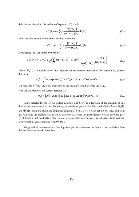
- Page 832 and 833: 1. ADS description A conceptual des
- Page 836 and 837: With the coupling LAHET + MCNP-DSP,
- Page 838 and 839: Figure 3. Comparison for 1 and 5 pu
- Page 841 and 842: MOLTEN SALTS AS POSSIBLE FUEL FLUID
- Page 843 and 844: 2. The fuel salt for MSB concept Ma
- Page 845 and 846: and minor actinides must be removed
- Page 847 and 848: 4. Container material studies 4.1 F
- Page 849 and 850: management. The major developments
- Page 851: REFERENCES [1] H.J. MacPherson, Dev
- Page 854 and 855: 1. Introduction The Energy Amplifie
- Page 856 and 857: Table 1. Main parameters of the EAD
- Page 858 and 859: Table 5. Neutron balance in the who
- Page 860 and 861: Table 7. Neutron flux distributions
- Page 862 and 863: Table 8. Displacement rates DPA/yea
- Page 865 and 866: DEEP UNDERGROUND TRANSMUTOR (PASSIV
- Page 867 and 868: passive state. By operating at a hi
- Page 869 and 870: I have proposed using an accelerato
- Page 871 and 872: Figure 1. Layout of deep undergroun
- Page 873 and 874: RADIATION CHARACTERISTICS OF PWR MO
- Page 875 and 876: Table 1. Radiotoxicity of actinides
- Page 877 and 878: RADIATION CHARACTERISTICS OF URANIU
- Page 879 and 880: Table 1. Radiotoxicity of actinides
- Page 881 and 882: INTERNATIONAL CO-OPERATION ON CREAT
- Page 883 and 884: an international base to combine ef
- Page 885:
• Second topic: interaction of pr
- Page 888 and 889:
1. Introduction The role of acceler
- Page 890 and 891:
MEPI within the framework of Projec
- Page 893 and 894:
NEW ORIGINAL IDEAS ON ACCELERATOR D
- Page 895 and 896:
During conceptual investigations of
- Page 897 and 898:
delay, interface and computer. The
- Page 899 and 900:
2. Channel-vessel design of ADS bla
- Page 901 and 902:
Table 1. Characteristics of the ful
- Page 903:
[14] Karavaev G.N., Kiselev G.V., M
- Page 906 and 907:
1. Introduction The problem of nucl
- Page 908 and 909:
Table 3. Radiotoxicity in americium
- Page 910 and 911:
Table 5. Characteristics of station
- Page 912 and 913:
1. Introduction The atomic power en
- Page 914 and 915:
of lead-bismuth target are given in
- Page 917 and 918:
CRITICAL AND SUB-CRITICAL GT-MHRs F
- Page 919 and 920:
Table 1. Basic GT-MHR reactor param
- Page 921 and 922:
Figure 2. Typical change of the ave
- Page 923 and 924:
Scenario S4. This case is actually
- Page 925 and 926:
Figure 3. A change in radiotoxicity
- Page 927:
[13] P. Goberis, Modelling of Innov
- Page 930 and 931:
1. Introduction The Nuclear Enginee
- Page 932 and 933:
Some simplifications have been made
- Page 934 and 935:
Figure 3. Velocity vectors Some of
- Page 936 and 937:
Figure 6. Temperature evolution at
- Page 938 and 939:
• Two main reasons can explain th
- Page 940 and 941:
1. Introduction Actually, we notice
- Page 942 and 943:
This problem can be solved by using
- Page 944 and 945:
The evaluations obtained in [2] hav
- Page 946 and 947:
REFERENCES [1] Management and Dispo
- Page 948 and 949:
1. Background Radiation background
- Page 950 and 951:
the long-term hazard of spent fuel,
- Page 952 and 953:
In a transmutation fuel cycle inclu
- Page 954 and 955:
Figure 4. Potential biological haza
- Page 956 and 957:
cooling prior to SF reprocessing an
- Page 958:
REFERENCES [1] White Book of Nuclea
- Page 961 and 962:
ORDER FORM OECD Nuclear Energy Agen