chapter 6 - Analog IC Design.org

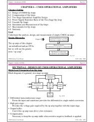
Chapter 6 – Section 2 (5/2/04) Page 6.2-24
Increasing the Magnitude of the Output Pole †
The magnitude of the output pole , p 2 , can be increased by introducing gain in the Miller
capacitor feedback path. For example,
M10
M11
Fig. 6.2-15B
M8
M12
C c
M9
V Bias
V DD
C gd6
C
r c
M7
ds8
+ +
v OUT
Iin R 1 V 1 Vs8 R 2 C 2
gm8Vs8
- -
M6
V SS
The resistors R 1 and R 2 are defined as
1
R 1 = g ds2 + g ds4 + g ds9
and R 2 =
g m6 V 1
g m6 V 1
+
V out
-
C gd6 C c
+
+
Iin R 1 V1 1
R 2 C 2
gm8 V s8
- g m8 V s8 -
1
g ds6 + g ds7
where transistors M2 and M4 are the output transistors of the first stage.
Nodal equations:
⎛ g
⎜ m8 sC c
⎞
⎡
⎤
⎟
⎢
⎥
I in = G 1 V 1 -g m8 V s8 = G 1 V 1 -⎜
⎟
⎝
g m8 + sC c
V out and 0 = g m6 V 1 + ⎢G ⎥
⎣ 2 +sC 2 + g m8sC c
g m8 +sC c
V out
⎠
+
V out
-
⎦
†
B.K. Ahuja, “An Improved Frequency Compensation Technique for CMOS Operational Amplifiers,” IEEE J. of Solid-State Circuits, Vol. SC-18,
No. 6 (Dec. 1983) pp. 629-633.
CMOS Analog Circuit Design © P.E. Allen - 2004
Chapter 6 – Section 2 (5/2/04) Page 6.2-25
Increasing the Magnitude of the Output Pole - Continued
Solving for the transfer function V out /I in gives,
V out
I in
⎛
⎜
= ⎜ ⎝
-g m6
⎞
⎟
⎟
⎠
G 1 G 2
⎣
⎢ ⎢⎢⎡
⎛
⎜
⎜
⎝
⎡ C
⎢ c
1 + s⎢
⎣
g + C 2
m8 G + C c
2
⎟
⎟
⎠
1 + sC c ⎞
g m8
⎤
⎥
⎥
⎦
G + g m6C c
2 G 1 G 2
⎛
⎜
+ s2
⎜ ⎝
C c C 2
g m8 G 2
Using the approximate method of solving for the roots of the denominator gives
-1
-6
p 1 = C c
g m8
+ C c
G 2
+ C 2
G 2
+ g m6C c
≈ g m6 r ds
2C c
G 1 G 2
and
p 2 ≈
- g m6r ds
2C c
6
C c C 2
g m8 G 2
= g m8r ds
2G 2
⎛
⎜
6 ⎜ ⎝
g m6
⎞
C 2
⎟
⎟
⎠
⎛
⎜
= ⎜ ⎝
g m8 r ds
⎞
3 |p 2 ’|
where all the various channel resistance have been assumed to equal r ds and p 2 ’ is the
output pole for normal Miller compensation.
Result:
Dominant pole is approximately the same and the output pole is increased by ≈ g m r ds .
⎟
⎟
⎠
⎞
⎟
⎟
⎠
⎦ ⎥⎥⎥⎤
CMOS Analog Circuit Design © P.E. Allen - 2004