Th`ese Marouan BOUALI - Sites personnels de TELECOM ParisTech

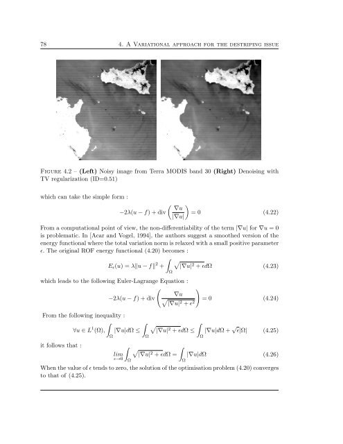
78 4. A Variational approach for the destriping issue
Figure 4.2 – (Left) Noisy image from Terra MODIS band 30 (Right) Denoising with
TV regularization (ID=0.51)
which can take the simple form :
−2λ(u − f) + div
( ) ∇u
= 0 (4.22)
|∇u|
From a computational point of view, the non-differentiability of the term |∇u| for ∇u =0
is problematic. In [Acar and Vogel, 1994], the authors suggest a smoothed version of the
energy functional where the total variation norm is relaxed with a small positive parameter
ɛ. The original ROF energy functional (4.20) becomes :
∫
√
E ɛ (u) =λ‖u − f‖ 2 + |∇u| 2 + ɛdΩ (4.23)
which leads to the following Euler-Lagrange Equation :
(
)
∇u
−2λ(u − f) + div √ = 0 (4.24)
|∇u| 2 + ɛ 2
From the following inequality :
∫
∫
∀u ∈ L 1 (Ω), |∇u|dΩ ≤
Ω
Ω
Ω
√
∫
|∇u| 2 + ɛdΩ ≤
Ω
|∇u|dΩ+ √ ɛ|Ω| (4.25)
it follows that :
√
∫
lim |∇u|
ɛ→0
∫Ω
2 + ɛdΩ = |∇u|dΩ (4.26)
Ω
When the value of ɛ tends to zero, the solution of the optimisation problem (4.20) converges
to that of (4.25).