Th`ese Marouan BOUALI - Sites personnels de TELECOM ParisTech

79
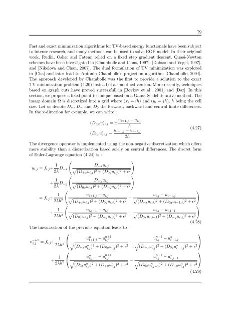
Fast and exact minimization algorithms for TV-based energy functionals have been subject
to intense research, and many methods can be used to solve ROF model. In their original
work, Rudin, Osher and Fatemi relied on a fixed step gradient descent. Quasi-Newton
schemes have been investigated in [Chambolle and Lions, 1997], [Dobson and Vogel, 1997],
and [Nikolova and Chan, 2007]. The dual formulation of TV minimization was explored
in [Cha] and later lead to Antonin Chambolle’s projection algorithm [Chambolle, 2004].
The approach developed by Chambolle was the first to provide a solution to the exact
TV minimization problem (4.20) instead of a smoothed version. More recently, techniques
based on graph cuts have proved successfull in [Boykov et al., 2001] and [Dar]. In this
section, we propose a fixed point technique based on a Gauss-Seidel iterative method. The
image domain Ω is discretized into a grid where (x i = ih) and (y i = jh), h being the cell
size. Let us denote D + , D − and D 0 the forward, backward and central finite differences.
In the x-direction for exemple, we can write :
(D ±x u) i,j = ± u i±1,j − u i,j
h
(D 0x u) i,j = u i+1,j − u i−1,j
2h
(4.27)
The divergence operator is implemented using the non-negative discretization which offers
more stability than a discretization based solely on central differences. The discret form
of Euler-Lagrange equation (4.24) is :
u i,j = f i,j + 1
2λ D −x
+ 1
2λ D −y
(
(
)
D +x u i,j
√
(D+x u i,j ) 2 +(D 0y u i,j ) 2 + ɛ 2
)
D +y u i,j
√
(D0x u i,j ) 2 +(D +y u i,j ) 2 + ɛ 2
(
)
= f i,j + 1
u i+1,j − u i,j
2λh 2 √
(D+x u i,j ) 2 +(D 0y u i,j ) 2 + ɛ − u i,j − u i−1,j
√ 2 (D−x u i,j ) 2 +(D 0y u i−1,j ) 2 + ɛ 2
(
)
+ 1
u i,j+1 − u i,j
2λh 2 √
(D0x u i,j ) 2 +(D +y u i,j ) 2 + ɛ − u i,j − u i,j−1
√ 2 (D0x u i,j−1 ) 2 +(D −y u i,j ) 2 + ɛ 2
(4.28)
The linearization of the previous equation leads to :
⎛
⎞
u n+1
i,j
= f i,j + 1
u
⎝
n i+1,j − un+1 i,j
u n+1
i,j
− u n i−1,j
2λh 2 − √
⎠
√(D +x u n i,j )2 +(D 0y u n i,j )2 + ɛ 2 (D −x u n i,j )2 +(D 0y u n i−1,j )2 + ɛ 2
⎛
⎞
+ 1
u
⎝
n i,j+1 − un+1 i,j
u n+1
i,j
− u n i,j−1
2λh 2 − √
⎠
√(D 0x u n i,j )2 +(D +y u n i,j )2 + ɛ 2 (D 0x u n i,j−1 )2 +(D −y u n i,j )2 + ɛ 2
(4.29)