- Page 1 and 2:
Chapter 1 INTRODUCTION TO CALCULUS
- Page 3 and 4:
y x 3 1 , if 3 6 t 6 0 t 6. A func
- Page 5 and 6:
What Is Calculus? Two simple geomet
- Page 7 and 8:
If a and b were radicals, squaring
- Page 9 and 10:
Exercise 1.1 PART A 1. Write the co
- Page 11 and 12:
Consider a curve y f 1x2 and a poi
- Page 13 and 14:
EXAMPLE 2 Tech Support For help gra
- Page 15 and 16:
The slope of the tangent at 13, 42
- Page 17 and 18:
INVESTIGATION 4 Tech Support For he
- Page 19 and 20:
4. Simplify each of the following d
- Page 21 and 22:
18. Copy the following figures. Dra
- Page 23 and 24:
A. Determine the average velocity o
- Page 25 and 26:
Instantaneous Velocity The velocity
- Page 27 and 28:
Solution a. C11002 10V100 1000 1
- Page 29 and 30:
Exercise 1.3 C PART A 1. The veloci
- Page 31 and 32:
f 1x2 f 1a2 15. Use the alternate
- Page 33 and 34:
. Use your results for part a to ap
- Page 35 and 36:
The graph shown on your calculator
- Page 37 and 38:
limits because, in each case, only
- Page 39 and 40:
11. For each function, sketch the g
- Page 41 and 42:
EXAMPLE 2 EXAMPLE 3 EXAMPLE 4 Using
- Page 43 and 44:
INVESTIGATION Here is an alternate
- Page 45 and 46:
In this section, we learned the pro
- Page 47 and 48:
A 11. Jacques Charles (1746-1823) d
- Page 49 and 50:
A second condition for continuity a
- Page 51 and 52:
d. The function F is not continuous
- Page 53 and 54:
x 3, if x 3 12. g1x2 e 2 k, if
- Page 55 and 56:
Key Concepts Review We began our in
- Page 57 and 58:
c. What is the present rate of chan
- Page 59 and 60:
16. Evaluate the limit of each diff
- Page 61 and 62:
Chapter 2 DERIVATIVES Imagine a dri
- Page 63 and 64:
2 4 5. Expand, and collect like te
- Page 65 and 66:
Section 2.1—The Derivative Functi
- Page 67 and 68:
For the Parabola f1x2 x 2 The slop
- Page 69 and 70:
Note that f 1t2 Vt is defined for
- Page 71 and 72:
EXAMPLE 6 Reasoning about different
- Page 73 and 74:
Exercise 2.1 PART A 1. State the do
- Page 75 and 76:
T 15. Match each function in graphs
- Page 77 and 78:
EXAMPLE 1 Applying the constant fun
- Page 79 and 80:
We conclude this section with the s
- Page 81 and 82:
EXAMPLE 6 Connecting the derivative
- Page 83 and 84:
x 1 8. Determine the slope of the
- Page 85 and 86:
Section 2.3—The Product Rule In t
- Page 87 and 88:
EXAMPLE 3 Selecting an efficient st
- Page 89 and 90:
EXAMPLE 6 Selecting a strategy to d
- Page 91 and 92:
PART B dy 5. Determine the value of
- Page 93 and 94:
9. Determine the equation of the ta
- Page 95 and 96:
EXAMPLE 1 Applying the quotient rul
- Page 97 and 98:
Exercise 2.4 PART A 1. What are the
- Page 99 and 100:
Section 2.5—The Derivatives of Co
- Page 101 and 102:
with respect to x is equal to the p
- Page 103 and 104:
EXAMPLE 7 Combining derivative rule
- Page 105 and 106:
Exercise 2.5 PART A 1. Given f 1x2
- Page 107 and 108:
Technology Extension: Derivatives o
- Page 109 and 110:
Key Concepts Review Now that you ha
- Page 111 and 112:
9. For what values of x does the cu
- Page 113 and 114:
24. At a manufacturing plant, produ
- Page 115 and 116:
Chapter 3 DERIVATIVES AND THEIR APP
- Page 117 and 118:
4. Determine the area of each figur
- Page 119 and 120:
Section 3.1—Higher-Order Derivati
- Page 121 and 122:
Motion on a Straight Line An object
- Page 123 and 124:
d. The object moves in a positive d
- Page 125 and 126:
EXAMPLE 5 Analyzing motion under gr
- Page 127 and 128:
Exercise 3.1 C K PART A 1. Explain
- Page 129 and 130:
T 12. A dragster races down a 400 m
- Page 131 and 132:
H. Repeat part D for the following
- Page 133 and 134:
Only t 3 is in the given interval,
- Page 135 and 136:
IN SUMMARY Key Ideas • The maximu
- Page 137 and 138:
T PART B 4. Using the algorithm for
- Page 139 and 140:
Mid-Chapter Review 1. Determine the
- Page 141 and 142:
Section 3.3—Optimization Problems
- Page 143 and 144:
For extreme values, set V¿1x2 0.
- Page 145 and 146:
Exercise 3.3 C PART A 1. A piece of
- Page 147 and 148:
a. Determine the dimensions that sh
- Page 149 and 150:
The revenue function is R1x2 17 0
- Page 151 and 152:
The minimal cost is approximately $
- Page 153 and 154:
T C 8. The fuel cost per hour for r
- Page 155 and 156:
CAREER LINK WRAP-UP Investigate and
- Page 157 and 158:
10. For each of the following cost
- Page 159 and 160: s1t2 t 26. Find the absolute maxi
- Page 161 and 162: Chapter 4 CURVE SKETCHING If you ar
- Page 163 and 164: 5. Determine the derivative of each
- Page 165 and 166: Section 4.1—Increasing and Decrea
- Page 167 and 168: dy Since this is a polynomial funct
- Page 169 and 170: IN SUMMARY Key Ideas • A function
- Page 171 and 172: 9. Each of the following graphs rep
- Page 173 and 174: Solution dy First determine dx . dy
- Page 175 and 176: Note that there is no value of x fo
- Page 177 and 178: EXAMPLE 4 Graphing the derivative g
- Page 179 and 180: 4. Find the x- and y-intercepts of
- Page 181 and 182: Section 4.3—Vertical and Horizont
- Page 183 and 184: The behaviour of the graph can be i
- Page 185 and 186: EXAMPLE 2 Expressing a polynomial f
- Page 187 and 188: When lim f 1x2 k or lim f 1x2 k,
- Page 189 and 190: For horizontal asymptotes, 3x f 1x2
- Page 191 and 192: Now let's consider the straight lin
- Page 193 and 194: Exercise 4.3 PART A 1. State the eq
- Page 195 and 196: 12. Use the features of each functi
- Page 197 and 198: 11. a. What does f ¿1x2 7 0 imply
- Page 199 and 200: From these investigations, we can m
- Page 201 and 202: Setting dy dx 0, we obtain 3 1x 2
- Page 203 and 204: The second derivative of f 1x2 is f
- Page 205 and 206: Exercise 4.4 K PART A 1. For each f
- Page 207 and 208: Section 4.5—An Algorithm for Curv
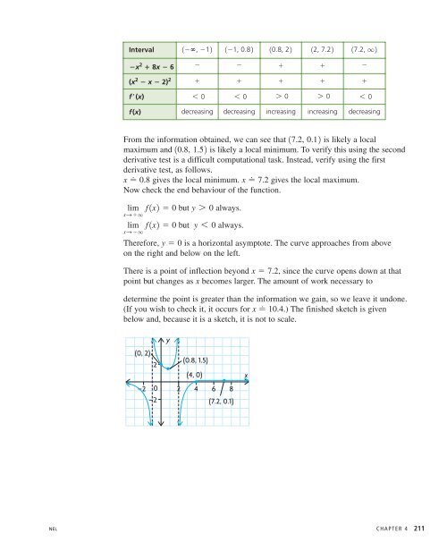
- Page 209: Therefore, by the second derivative
- Page 213 and 214: K A 1x PART B 4. Use the algorithm
- Page 215 and 216: Key Concepts Review In this chapter
- Page 217 and 218: 5. For each of the following, check
- Page 219 and 220: 17. If f 1x2 x3 8 , determine the
- Page 221 and 222: Chapter 5 DERIVATIVES OF EXPONENTIA
- Page 223 and 224: Radian Measure A radian is the meas
- Page 225 and 226: 5. Convert the following angles to
- Page 227 and 228: Section 5.1—Derivatives of Expone
- Page 229 and 230: From the investigation, you should
- Page 231 and 232: EXAMPLE 4 Connecting the derivative
- Page 233 and 234: A C PART B 6. Determine the equatio
- Page 235 and 236: Section 5.2—The Derivative of the
- Page 237 and 238: In general, for the exponential fun
- Page 239 and 240: Solution a. January 1, 1900, is exa
- Page 241 and 242: Section 5.3—Optimization Problems
- Page 243 and 244: The average revenue to the company
- Page 245 and 246: Exercise 5.3 PART A 1. Use graphing
- Page 247 and 248: 12. Find the maximum and minimum va
- Page 249 and 250: 9. The rapid growth in the number o
- Page 251 and 252: INVESTIGATION 2 A.Using your graphi
- Page 253 and 254: With practice, you will learn how t
- Page 255 and 256: We evaluate f 1x2 at the critical n
- Page 257 and 258: A T 6. Determine the absolute extre
- Page 259 and 260: Derivatives of Composite Functions
- Page 261 and 262:
CAREER LINK WRAP-UP Investigate and
- Page 263 and 264:
Review Exercise 1. Differentiate ea
- Page 265 and 266:
18. The position of a particle is g
- Page 267 and 268:
Chapter 5 Test dy 1. Determine the
- Page 269 and 270:
8. Use algebraic methods to evaluat
- Page 271 and 272:
f 1x2 142e 5x1 24. For each functi
- Page 273 and 274:
Review of Prerequisite Skills In th
- Page 275 and 276:
CAREER LINK Investigate CHAPTER 6:
- Page 277 and 278:
What is a Vector? A vector is a mat
- Page 279 and 280:
EXAMPLE 1 B A E D C Connecting vect
- Page 281 and 282:
A K B 5. Given the vector AB ! as s
- Page 283 and 284:
Section 6.2—Vector Addition In th
- Page 285 and 286:
the overall magnitude would be equa
- Page 287 and 288:
Solution c b a a - b + c a - b c a
- Page 289 and 290:
W N S E The vectors are drawn so th
- Page 291 and 292:
Exercise 6.2 PART A 1. The vectors
- Page 293 and 294:
10. a. In ! the ! example ! involvi
- Page 295 and 296:
0 0 The previous example illustrate
- Page 297 and 298:
Solution a. 30˚ y x 2x-y 2x -y 30
- Page 299 and 300:
Solution Draw a sketch and determin
- Page 301 and 302:
8. The two vectors a ! and b ! are
- Page 303 and 304:
Section 6.4—Properties of Vectors
- Page 305 and 306:
Demonstrating the distributive law
- Page 307 and 308:
IN SUMMARY Key Idea • Properties
- Page 309 and 310:
Mid-Chapter Review 1. ABCD is a par
- Page 311 and 312:
Section 6.5—Vectors in R 2 and R
- Page 313 and 314:
Right-Handed System of Coordinates
- Page 315 and 316:
Solution a. A16, 0, 02 is a point o
- Page 317 and 318:
There is one further observation th
- Page 319 and 320:
C A 14. a. What is the equation of
- Page 321 and 322:
R 2 EXAMPLE 1 Representing vectors
- Page 323 and 324:
EXAMPLE 2 Representing the sum and
- Page 325 and 326:
EXAMPLE 5 Calculating the magnitude
- Page 327 and 328:
A 10. Parallelogram is determined b
- Page 329 and 330:
EXAMPLE 1 Representing vectors in R
- Page 331 and 332:
. Using components, a ! b ! c !
- Page 333 and 334:
IN SUMMARY Key Ideas • In R 3 , i
- Page 335 and 336:
Section 6.8—Linear Combinations a
- Page 337 and 338:
In R 2 , it is possible to take any
- Page 339 and 340:
Geometrically, the linear combinati
- Page 341 and 342:
IN SUMMARY Key Ideas • In R 2 , O
- Page 343 and 344:
CAREER LINK WRAP-UP Investigate and
- Page 345 and 346:
Review Exercise 1. Determine whethe
- Page 347 and 348:
15. A rectangular prism measuring 3
- Page 349 and 350:
Chapter 6 Test 1. The vectors a ! ,
- Page 351 and 352:
Review of Prerequisite Skills In th
- Page 353 and 354:
Section 7.1—Vectors as Forces The
- Page 355 and 356:
of 6 cm, also pointing east. The ve
- Page 357 and 358:
is drawn approximately to scale, an
- Page 359 and 360:
The magnitude of the vertical compo
- Page 361 and 362:
! T1 sin 105° 1961sin 45°2 T ! 1
- Page 363 and 364:
49 34 30 cos CBA 1 cos CBA 2 120
- Page 365 and 366:
C T f 3 40 N O 35 N 45° 30 N f 2 2
- Page 367 and 368:
Solution We start by drawing positi
- Page 369 and 370:
v a v + w w 20 triangles, Solving t
- Page 371 and 372:
A T C 9. A small airplane has an ai
- Page 373 and 374:
Perhaps the most important observat
- Page 375 and 376:
If we look at the right-angled tria
- Page 377 and 378:
Solution Consider the following dia
- Page 379 and 380:
A T 10. What is the value of the do
- Page 381 and 382:
Expanding, we get b 2 1 2a 1 b 1
- Page 383 and 384:
. 0 a ! 0 2 @b ! 112 2 122 2 142
- Page 385 and 386:
One of the most important propertie
- Page 387 and 388:
4. a. From the set of vectors e11,
- Page 389 and 390:
Mid-Chapter Review 1. a. If 0 a ! 0
- Page 391 and 392:
Section 7.5—Scalar and Vector Pro
- Page 393 and 394:
EXAMPLE 1 Reasoning about the chara
- Page 395 and 396:
x EXAMPLE 3 z P (2, 1, 4) g b a O(0
- Page 397 and 398:
EXAMPLE 4 Calculating a specific di
- Page 399 and 400:
IN SUMMARY Key Idea • A projectio
- Page 401 and 402:
B C 12. In the diagram shown, ^ ABC
- Page 403 and 404:
a 3 b, k = 1 O b 3 a, k = -1 b a is
- Page 405 and 406:
If we carry out an identical proced
- Page 407 and 408:
EXAMPLE 2 Calculating cross product
- Page 409 and 410:
K A C T 4. Calculate the cross prod
- Page 411 and 412:
EXAMPLE 1 Using the dot product to
- Page 413 and 414:
. We start by constructing position
- Page 415 and 416:
EXAMPLE 4 Using the cross product t
- Page 417 and 418:
CAREER LINK WRAP-UP Investigate and
- Page 419 and 420:
Review Exercise 1. Given that a !
- Page 421 and 422:
18. For the vectors m ! 1 V3, 2, 3
- Page 423 and 424:
Chapter 7 Test 1. Given the vectors
- Page 425 and 426:
Review of Prerequisite Skills In th
- Page 427 and 428:
CAREER LINK Investigate CHAPTER 8:
- Page 429 and 430:
Both of these vectors can be multip
- Page 431 and 432:
c. If the point Q121, 232 lies on t
- Page 433 and 434:
In this section, the vector and par
- Page 435 and 436:
C K A T 6. a. If the equation of a
- Page 437 and 438:
EXAMPLE 1 Representing the Cartesia
- Page 439 and 440:
It is not possible, in this case, t
- Page 441 and 442:
AP ! 1x 4, y 1222 1x 4, y 22.
- Page 443 and 444:
u cos 1 a 3 12 1 10 21 25 2 b u
- Page 445 and 446:
A T 10. For each pair of lines, det
- Page 447 and 448:
is its direction vector. If represe
- Page 449 and 450:
EXAMPLE 4 Representing the equation
- Page 451 and 452:
C A T 6. a. Determine parametric eq
- Page 453 and 454:
13. The Cartesian equation of a lin
- Page 455 and 456:
s t s(1, 2, 1) t(0, 2, 1), s, tR P
- Page 457 and 458:
After deriving vector and parametri
- Page 459 and 460:
EXAMPLE 4 Representing the equation
- Page 461 and 462:
A K T 7. a. Determine parameters co
- Page 463 and 464:
To derive the equation of this plan
- Page 465 and 466:
A number of observations can be mad
- Page 467 and 468:
When we considered lines in R 2 , w
- Page 469 and 470:
IN SUMMARY Key Idea • The Cartesi
- Page 471 and 472:
Section 8.6—Sketching Planes in R
- Page 473 and 474:
EXAMPLE 2 Representing the graph of
- Page 475 and 476:
EXAMPLE 5 Graphing planes whose Car
- Page 477 and 478:
IN SUMMARY Key Idea • A sketch of
- Page 479 and 480:
CAREER LINK WRAP-UP Investigate and
- Page 481 and 482:
Review Exercise 1. Determine vector
- Page 483 and 484:
20. Calculate the acute angle that
- Page 485 and 486:
Chapter 8 Test 1. a. Given the poin
- Page 487 and 488:
Review of Prerequisite Skills In th
- Page 489 and 490:
CAREER LINK Investigate CHAPTER 9:
- Page 491 and 492:
4 13 s2 211 4s2 12 8s2 8 0 1
- Page 493 and 494:
Method 2: Again, this result can be
- Page 495 and 496:
We can now select any two of the th
- Page 497 and 498:
IN SUMMARY Key Ideas • Line and p
- Page 499 and 500:
A T 11. a. Show that the lines and
- Page 501 and 502:
equations. Since the lines would be
- Page 503 and 504:
Solution 1: Interchange equations 1
- Page 505 and 506:
Substituting into the second equati
- Page 507 and 508:
1: Multiply equation 1 by k, and ad
- Page 509 and 510:
K C PART B 4. Solve each system of
- Page 511 and 512:
Section 9.3—The Intersection of T
- Page 513 and 514:
If we had solved the system using e
- Page 515 and 516:
then x 3s 1. Now it is a matter o
- Page 517 and 518:
Exercise 9.3 C K PART A 1. A system
- Page 519 and 520:
Mid-Chapter Review 1. Determine the
- Page 521 and 522:
Section 9.4—The Intersection of T
- Page 523 and 524:
1: Create two new equations, 4 and
- Page 525 and 526:
Thus, 7y 5t 3. Dividing by 7, we g
- Page 527 and 528:
Inconsistent Systems for Three Equa
- Page 529 and 530:
Therefore, we can choose ! ! ! m 1
- Page 531 and 532:
Exercise 9.4 PART A 1. A student is
- Page 533 and 534:
9. Solve each system of equations u
- Page 535 and 536:
Section 9.5—The Distance from a P
- Page 537 and 538:
EXAMPLE 1 Calculating the distance
- Page 539 and 540:
In triangle PQR, sin u d @ QP ! @
- Page 541 and 542:
Exercise 9.5 PART A 1. Determine th
- Page 543 and 544:
Section 9.6—The Distance from a P
- Page 545 and 546:
It is also possible to use the dist
- Page 547 and 548:
p 1 p 2 U V d L 1 : r = (-2, 1, 0)
- Page 549 and 550:
The required distance between the t
- Page 551 and 552:
K A T PART B 2. Determine the follo
- Page 553 and 554:
Review Exercise 1. The lines 2x y
- Page 555 and 556:
14. You are given the lines , and r
- Page 557 and 558:
Chapter 9 Test 1. a. Determine the
- Page 559 and 560:
P(1, -2, 4) Q P9 2x - 3y - 4z + 66
- Page 561 and 562:
29. A line that passes through the
- Page 563 and 564:
Solution a. Differentiate both side
- Page 565 and 566:
Exercise PART A 1. State the chain
- Page 567 and 568:
dA b. To determine differentiate A
- Page 569 and 570:
1 16 dh dt Therefore, at the momen
- Page 571 and 572:
11. Two cyclists depart at the same
- Page 573 and 574:
Solution a. y ln15x2 Using the cha
- Page 575 and 576:
x1x 42 0 x 4 or x 0 But x 0 is
- Page 577 and 578:
The Derivatives of General Logarith
- Page 579 and 580:
The Derivative of a Composite Funct
- Page 581 and 582:
To solve this, we take the natural
- Page 583 and 584:
Exercise PART A 1. Differentiate ea
- Page 585 and 586:
y eliminating unknowns. In Example
- Page 587 and 588:
Properties of a Matrix in Row-Echel
- Page 589 and 590:
Exercise PART A 1. Write an augment
- Page 591 and 592:
12. Determine the equation of the p
- Page 593 and 594:
1 0 0 18 4 (row 3) row 1 £ 0 1 0
- Page 595 and 596:
Finally, convert the entry in the s
- Page 597 and 598:
Review of Technical Skills Appendix
- Page 599 and 600:
3 Evaluating a Function 1. Enter th
- Page 601 and 602:
7 Making a Table of Differences To
- Page 603 and 604:
4. Cursor along the curve to any po
- Page 605 and 606:
5. Display and analyze the results.
- Page 607 and 608:
14 Graphing a Trigonometric Functio
- Page 609 and 610:
2. Enter the second equation. Press
- Page 611 and 612:
Use either the calculator keypad or
- Page 613 and 614:
20 Graphing the Derivative of a Fun
- Page 615 and 616:
4. Create a function. Right-click t
- Page 617 and 618:
composition: the process of combini
- Page 619 and 620:
G geometric vectors: vectors that a
- Page 621 and 622:
ationalizing the denominator: the p
- Page 623 and 624:
Answers Chapter 1 0 0 0 0 0 Review
- Page 625 and 626:
d. about 1 e. about 7 8 f. no tang
- Page 627 and 628:
d. 13. m 3; b 1 14. a 3, b 2, c
- Page 629 and 630:
Review Exercise, pp. 56-59 1. a. 3
- Page 631 and 632:
19. a. y 7 b. y 5x 5 c. y 18x 9
- Page 633 and 634:
20. a. 34.3 m> s b. 39.2 m> s c. 54
- Page 635 and 636:
17. a. 100 bacteria b. 1200 bacteri
- Page 637 and 638:
11. a. b. 160x y 16 0 60x y 61
- Page 639 and 640:
3. 1 2x 4. a. x 2 15x 6 b. 6012x
- Page 641 and 642:
14. t 1 s; away 15. a. s1t2 kt 2
- Page 643 and 644:
14. a. triangle side length 0.96 cm
- Page 645 and 646:
Review Exercise, pp. 156-159 11. 20
- Page 647 and 648:
c. i. ii. iii. d. i. ii. iii. 5 4 3
- Page 649 and 650:
. local minimum: 11.41, 39.62, loca
- Page 651 and 652:
2. increasing: x 6 1 and x 7 2, dec
- Page 653 and 654:
to a zero of its derivative, the nu
- Page 655 and 656:
7. (-2, 10) 10 8 y 10. a. 8 y e. 4
- Page 657 and 658:
4. hole at x 2; large and negative
- Page 659 and 660:
sin x b. 1 sin 2 tan x sec x x L
- Page 661 and 662:
12. a. no maximum or minimum value
- Page 663 and 664:
Review Exercise, pp. 263-265 1. a.
- Page 665 and 666:
x 2. 5. a. 19 000 fish> year b. 23
- Page 667 and 668:
Section 6.1, pp. 279-281 6. a. b. c
- Page 669 and 670:
17. P G 4. Answers may vary. For ex
- Page 671 and 672:
11. a. AG ! a ! b ! c ! , b. AG
- Page 673 and 674:
d. OD ! 11, 1, 12 (0, 0, 1) (1, 0,
- Page 675 and 676:
Section 6.7, pp. 332-333 1. a. 1i !
- Page 677 and 678:
24. 25. a. 0a ! b. 0a ! 0 2 0b !
- Page 679 and 680:
. Since the equilibrant is directed
- Page 681 and 682:
7. a. scalar projection: 0, vector
- Page 683 and 684:
2. a. 3 b. 7 c. 43 d. 217 e. 5 f. 1
- Page 685 and 686:
cos A 1 cos B 1 cos C 1 area of t
- Page 687 and 688:
. r ! 11, 1, 02 t10, 1, 12, tR; x
- Page 689 and 690:
2. 12, 3, 42 3. P must lie on plane
- Page 691 and 692:
25. A plane has two parameters, bec
- Page 693 and 694:
coincident with the plane, meaning
- Page 695 and 696:
Mid-Chapter Review, pp. 518-519 1.
- Page 697 and 698:
8. a. b. y 1 z 1 4 , 2 c. x 3t
- Page 699 and 700:
10. vector equation: r ! 10, 0, 42
- Page 701 and 702:
. 23. a. b. 2a 1 2 b a 6 7 , 2 7 ,
- Page 703 and 704:
16. 17. 18. 19. 2 3 4 m>min 144 m>m
- Page 705 and 706:
ln x 1 e. ln 2 4x 1 x ln 13x 2 2
- Page 707 and 708:
Index A Absolute extrema, 130, 132,
- Page 709:
normal, 461-469, 486, 512, 524 para