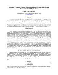
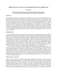
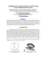
fkm∈{ 0,1,2, !} − { }, = 2 ,m ∈{ !}{ 0,1,2, !} { }, 2 1,m { !}⎧ 2k k m n m⎪ f c,⎪ 2 mand 1,2,3, ,= ⎨⎪ 2k+ 1 k∈ − m n = m+⎪fc,⎩2m+ 1 and ∈ 0,1,2, .As the locations of the nulls indicate, the behavior of Ŝdepends on whether one is considering full cycles ( n = 2m)or half cycles ( n = 2m+ 1) of the sine function inEquation (20a). In either case, the power spectral densityhas a value of ⎡⎣ns( ) 20 4 f c ⎤⎦ at f c , which is close but notequal to a local maximum. For very broadband signals( n ≤ 10 ), the local maximum differs significantly from f c ,although it lies between f c and one of its two nearest nullfrequencies. As n increases, the local maximum approachesf c . In particular, this local maximum is the global maximum,f M , for even n, and f M is 0.837470 f c for n = 2 (onecycle), 0.998480 f c for n = 20 (10 cycles), and0.999985 f c for n = 200 (100 cycles). When n is odd2( = 2m+ 1),Ŝ has a dc component of ⎡⎣s( ) 20 π fc⎤⎦ ,which is significant for small m. Specifically, the ratio of22Ŝ at 0 Hz to Ŝ at f c is 1.62 (2.1 dB) for m = 0 , is 0.18( −7.4dB) for m = 1 , and is 0.06 ( −11.9dB) for m = 2 . Asm increases, the dc component becomes negligible, and theglobal maximum approaches f c .2The portion of the plot of a power spectral densitybetween two nulls that don’t include f M is called a sidelobe.The height of each sidelobe is a function of n and the orderof the sidelobe (that is, first, second, third, etc., sidelobes).In some cases, one or more sidelobes exceed the chosenpower threshold, resulting in multiple pairs of crossingpoints at the threshold. If only the crossing points nearestthe global maximum are used to determine f l and f h , theresulting bandwidth will not accurately represent thefrequency band occupied by this signal. For widebandsignals ( n ≤ 10 ), a significant part of the spectrum would belost by filtering above the first null, which would severelydegrade the information content of the signal. In contrast toa spectrum consisting of a superposition of narrowbandsignals, the notches in the spectrum of a wideband signal donot separate the spectra of sub-signals. Actually, someapplications of UWB communication (for example,broadband over power lines) intentionally design thesenotches to protect other narrowband signals and services.Consequently, the lowest and the highest crossing points,{ f } and sup{ f }inf lh , may be appropriate for determiningthe power-level bandwidth to avoid inaccuratelycharacterizing the bandwidths of wideband signals andsignals with spectral notches.To make the preceding discussion more concrete, theone-cycle sine (a UWB signal) and its normalized powerspectral density are plotted in Figure 4. The peak powerlevel of the first sidelobe between 2 f c and 3 f c is 18.12 dBbelow the absolute maximum value at 0.837470 f c in themain lobe between 0 Hz and 2 f c . On inspecting Figure 4b,one clearly sees that the −20dB line intersects the curve infour places. Consequently, B 20dB includes a significantportion of the first sidelobe. A similar situation occurs forB 99EB , since the main lobe contains only 98.93 % of thesignal energy (Table 5). On comparing the classificationsin Table 5, one observes that the bandwidth measures formthree groups: Group 1 ( B 3dB and B 90EB ) contains only themain lobe and classifies the signal as UWB/SHB; Group 2( B 20dB , B RMS , and B 99EB ) includes the first sidelobe andclassifies the signal as UWB/HB; and Group 3 ( B 10dB ) actslike an interface between Groups 1 and 2, since it classifiesthe signal as UWB/HB but contains only the main lobe.The preceding example illustrates thatcharacterizations of wideband and UWB signals in thefrequency domain require more parameters than narrowbandsignals. For narrowband signals, one can assume that asingle peak, containing almost the entire signal energy,dominates the spectrum. In contrast, the signal energy ofwideband/UWB signals is spread over an extremely widerange of frequencies, wherein the amplitude can varysignificantly (notches and multiple peaks). Consequently,using only the calculated bandwidths of wideband andFigure 4a. A time-domain representation of a onecyclesine.Figure 4b. A frequency-domain representationof a one-cycle sine.22The<strong>Radio</strong> <strong>Science</strong> <strong>Bulletin</strong> No <strong>313</strong> (<strong>June</strong>, <strong>2005</strong>)
Bandwidths f l / f c f h / f c B F Classification E relB 3dB 0.410 1.30 1.04 UWB / SHB 79.05 %B 10dB 0.170 1.65 1.63 UWB / HB 97.18 %B 20dB 0.050 2.62 1.93 UWB / HB 99.58 %B RMS 0.000 2.24 2.00 UWB / HB 99.04 %B 90EB 0.305 1.445 1.30 UWB / SHB 90 %B 99EB 0.051 2.215 1.91 UWB / HB 99 %Table 5. Classification of the one-cycle sine for six bandwidth definitions.UWB signals provides incomplete and fragmentarycharacterizations of the signals. Therefore, additionalparameters, like the waviness (ripple), which characterizesthe variation of the amplitude in the specified band, areneeded for a more complete understanding of signalcharacterizations.5.4 Linear Frequency-ModulatedSine (Chirp)2⎧ ( f − fc)− jπ⎪ fcµ⎨e ⎡⎣−C( x1) − jS( x1) + C( x2) + jS( x2)⎤⎦⎪⎩2( f + fc)⎫jπfcµ⎪−e ⎡⎣C( x3) − jS( x3) − C( x4) + jS( x4)⎤⎬ ⎦ ,(21b) ⎪⎭A classical radar signal is the linear frequencymodulated(LFM) waveform, which is implemented bymodulating the sine function to increase the signalbandwidth. This waveform and pulse compression in aradar receiver are used to simultaneously obtain the energyof a long-duration signal and the resolution of a high-energyshort-duration signal. Pulse compression “is implementedin high-power radar applications that are limited by voltagebreakdown if a short-pulse were to be used” [13]. The linearfrequency-modulated waveform, also called chirpmodulation, sweeps linearly over a frequency band duringa given time interval, and is given by [14]⎡ ⎛ 1 2 ⎞⎤s() t = s0sin ⎢2π fc⎜t+ µ t ⎟ ⎡σ() t −σ( t−Tn)⎤2⎥⎣ ⎦,⎣ ⎝ ⎠⎦(21a)with the pulse durationTn1 ⎛ nµ⎞= − 1+ 1+µ ⎜f ⎟,⎝c ⎠where n is the number of half cycles, s 0 is the nominalamplitude, and m is the chirp rate. For 0 ≤t≤ Tn, theinstantaneous frequency, f () t , is f c + µ t , which variesfrom f c (the carrier and starting frequency) to fc+ µ Tn.Evaluating the Fourier transform yields1Sˆ( f ) =2j 2f c µwith2cf − f + nfcµx1 = 2,f µxx3 2cf − f= ,f µ2 2cc2cf + f + nfcµ= ,f µxcf + f= ,f µ4 2ccwhere C()x and S()x are the Fresnel integralsx⎛π2 ⎞C() x = ∫ cos⎜ y ⎟dy⎝ 2 ⎠,0x⎛π2 ⎞S( x) = ∫ sin ⎜ y ⎟dy.⎝ 2 ⎠0The relatively constant run of the in-band magnitudespectrum is the main advantage of the linear frequencymodulatedwaveform for practical applications. TheThe<strong>Radio</strong> <strong>Science</strong> <strong>Bulletin</strong> No <strong>313</strong> (<strong>June</strong>, <strong>2005</strong>) 23
- Page 1 and 2: Radio Science BulletinISSN 1024-453
- Page 3 and 4: EditorialJune in December?Yes, this
- Page 5 and 6: URSI Accounts 2004In 2004, a year p
- Page 7 and 8: EURO EUROA2) Routine Meetings 7,315
- Page 9 and 10: URSI AWARDS 2005The URSI Board of O
- Page 11 and 12: Guest Editors’ RemarksOn February
- Page 13 and 14: UWB and the corresponding signal pa
- Page 15 and 16: Radar / CommunicationsBand TypeElec
- Page 17 and 18: of the spectrum is required to comp
- Page 19 and 20: Bandwidths f l / GHz f h / GHz B F
- Page 21: Figure 3a. A time-domain representa
- Page 25 and 26: Bandwidth f l / f c f h / f c B F C
- Page 27 and 28: Quantitative Comparison BetweenMatr
- Page 29 and 30: Next, construct the ‘filtered’
- Page 31 and 32: whereH[ P ] [ U][ ][ V] ,N= Σ (27)
- Page 33 and 34: CPU Time [sec]250200150100MPMSS1SS2
- Page 35 and 36: -10-20MPMSS1SS2-30-40RMSE [dB]-50-6
- Page 37 and 38: RMSE [dB]-45-50-55-60-65-70MPMSS1SS
- Page 39 and 40: An Ultra-Compact Impulse-Radiating
- Page 41 and 42: Figure 3. UCIRA-1 splitter/balun.th
- Page 43 and 44: Figure 9. UCIRA-2 in stowed configu
- Page 45 and 46: activated first in the deployment s
- Page 47 and 48: Figure 20. Theoretical gain ofUCIRA
- Page 49 and 50: Triennial Reports CommissionsCOMMIS
- Page 51: y the Special Section Editors, and
- Page 55 and 56: 3.2 Activities of URSI-Commission C
- Page 57 and 58: It already has been decided that th
- Page 59 and 60: SCOR (Scientific Committee on Ocean
- Page 61 and 62: COMMISSION GThis triennium report w
- Page 63 and 64: GNSS-LEO occultation is a very impo
- Page 65 and 66: CPEA Contacts: Shoichiro Fukao, Pro
- Page 67 and 68: The group wishes to continue as an
- Page 69 and 70: total of 109 oral papers (24 thereo
- Page 71 and 72: surface, to compensate for the rema
- Page 73 and 74:
XXVIIIth General AssemblyNEWLY ELEC
- Page 75 and 76:
Décide1. d’accepter l’invitati
- Page 77 and 78:
satellite observation, bottomside s
- Page 79 and 80:
ETTC ‘05EUROPEAN TEST AND TELEMET
- Page 81 and 82:
IRI 2005 WORKSHOPNEW SATELLITE AND
- Page 83 and 84:
financial and logistics issues conn
- Page 85 and 86:
CONFERENCE ANNOUNCEMENTS36 TH COSPA
- Page 87 and 88:
December 2006APMC 2006 - 2006 Asia-
- Page 89 and 90:
The Journal of Atmospheric and Sola
- Page 91 and 92:
SCIENTIFIC COMMISSIONSCommission A
- Page 93 and 94:
Commission E : Electromagnetic Nois
- Page 95 and 96:
Commission J : Radio AstronomyChair
- Page 97 and 98:
URSI MEMBER COMMITTEESAUSTRALIA Pre
- Page 99 and 100:
ALPHABETICAL INDEX AND CO-ORDINATES
- Page 101 and 102:
BRUSSAARD, Prof. dr.ir. G., Radicom
- Page 103 and 104:
FEICK, Dr. R., Depto. de Electronic
- Page 105 and 106:
SAUDI ARABIA, Tel. +966 1-4883555/4
- Page 107 and 108:
E-mail loulee@nspo.gov.tw (94)LEE,
- Page 109 and 110:
O’DROMA, Dr. M., Dept. of Electri
- Page 111 and 112:
+30 2310 998161, Fax +30 2310 99806
- Page 113 and 114:
TURSKI, Prof. A., ul. Krochmalna 3
- Page 115 and 116:
Information for authorsContentThe R