Radio Science Bulletin 313 - June 2005 - URSI

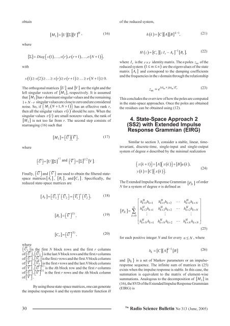
obtainof the reduced system,wherewith[ M ] [ U][ ][ V]1H= Σ , (16)[] Σ = Diag ⎡s() ! s() r e( r + )!e( N + )⎣1, , , 1, , 1 ⎤⎦,() ( ) () ( ) ( )s 1 ≥ s 2 ≥…≥ s r ≥ e r+ 1 ≥…≥ e N + 1 ≥0.V are the right and the, respectively. It is assumed1 has r dominant singular values and the remaining1+ N -rsingular values are close to zero and are considerednoise. So, if ⎡⎣M1 ( N + 1, N + 1)⎤⎦ has an effective rank r,then all the singular values ei () should be zero. When thesingular values ei () are small nonzero values, the rank of[ M 1]is not too far from r. The second step consists ofrearranging (16) such thatThe orthogonal matrices [ U ] and [ ]left singular vectors of [ M 1]that [ M ]where[ ]M ⎣U⎦⎣V⎦1 = ⎡ ⎤⎡ ⎤,[ U][ ] 1/2and 1/2⎡V⎤=Σ[] [] V .⎡⎣U⎤= ⎦ Σ⎣⎦(17)Finally, ⎡⎣U⎤⎦ and ⎡ ⎣ V ⎤ ⎦ are used to obtain the filtered statespacematrices[ A r], [ B r], and[ C r]. Specifically, thereduced state-space matrices are[ A ] = ⎡U1⎤ ⎡U2⎤=⎡V1⎤ ⎡V2 ⎤ ,r+ +⎣ ⎦ ⎣ ⎦ ⎣ ⎦ ⎣ ⎦[ B ]r[ C ]r= ⎡⎣V⎤⎦= ⎡⎣U⎤⎦(1),(1),(18)(19)(20)where⎡⎣U 1 ⎤⎦is the first N block rows and the first r columnsof ⎡⎣U⎤⎦ , ⎡⎣U 2 ⎤⎦ is the last N block rows and the first r columnsof ⎡⎣U⎤⎦ , ⎡⎣V 1⎤⎦is the first r rows and the first N block columnsof ⎡⎣V⎤⎦ , V 2 ⎤⎦is the first r rows and the last N block columnsof ⎡⎣V⎤⎦ , () i⎡⎣U⎤⎦ is the ith block row and the first r columnsof ⎡⎣U⎤⎦ , () i⎡⎣V⎤⎦ is the first r rows and the ith block columnof ⎡⎣V⎤⎦ Ḃy using these state-space matrices, one can generatethe impulse response h and the system transfer function Hk() [ ][ ][ ] 1 ,h k = C A B −(21)−1() [ ][ ] [ ]H z = C zI − A B , (22)r r r rwhere I r is the r× r identity matrix. The n poles z m of thereduced system ( 1 ≤m≤ n)are the eigenvalues of the statematrix [ A r]and correspond to the damping coefficientsand the frequencies in the s domain through the relationship( m j m)Tsm = +(23)z e α ωThis concludes the overview of how the poles are computedin the state-space approaches. Once the poles are obtainedthe residues can be obtained using (12).4. State-Space Approach 2(SS2) with Extended ImpulseResponse Grammian (EIRG)Similar to section 3, consider a stable, linear, timeinvariant,discrete-time, single-input and single-outputsystem of degree n described by the minimal realizationx( k + ) = [ A] x() k + [ B] u()k() = [ ] ⎡ () ⎤.⎡⎣ 1 ⎤⎦ ⎡⎣ ⎤⎦,y k C ⎣x k ⎦The Extended Impulse Response Grammian [ P ]N for a system of degree n is defined as[ P ]NN(24)of order⎡ H H Hhk+ 1hk+ 1 hk+ 1hk+ 2 " hk 1h⎤+ k+N⎢⎥∞ H H H⎢hk+ 2hk+ 1 hk+ 2hk+ 2 " hk+ 2hk+N ⎥= ∑ ⎢ ⎥k=0 ⎢ # # # ⎥⎢ H H Hhk+ Nhk+ 1 hk+ Nhk+ 2 hk+ Nh⎥⎣" k+N⎦(25)for each positive integer N and for every n≤N , whereand { }kk−1[ ][ ] [ ]h = C A B(26)h k is a set of Markov parameters or an impulseresponsesequence. The infinite sum of matrices in (25)exists when the impulse response is stable. In this case, thesummation is equivalent to the matrix of element-wisesummations. Analogous to the decomposition of [ M 1]in(16), the SVD of the Extended Impulse Response Grammian(EIRG) is30TheRadio Science Bulletin No 313 (June, 2005)