Radio Science Bulletin 313 - June 2005 - URSI

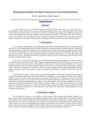
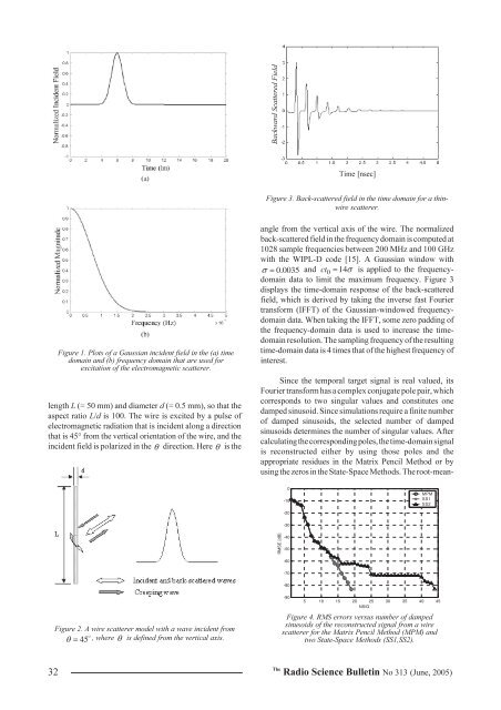
Backward Scattered FieldTime [nsec]Figure 3. Back-scattered field in the time domain for a thinwirescatterer.Figure 1. Plots of a Gaussian incident field in the (a) timedomain and (b) frequency domain that are used forexcitation of the electromagnetic scatterer.length L (= 50 mm) and diameter d (= 0.5 mm), so that theaspect ratio L/d is 100. The wire is excited by a pulse ofelectromagnetic radiation that is incident along a directionthat is 45° from the vertical orientation of the wire, and theincident field is polarized in the θ direction. Here θ is theangle from the vertical axis of the wire. The normalizedback-scattered field in the frequency domain is computed at1028 sample frequencies between 200 MHz and 100 GHzwith the WIPL-D code [15]. A Gaussian window withσ = 0.0035 and ct0 = 14σis applied to the frequencydomaindata to limit the maximum frequency. Figure 3displays the time-domain response of the back-scatteredfield, which is derived by taking the inverse fast Fouriertransform (IFFT) of the Gaussian-windowed frequencydomaindata. When taking the IFFT, some zero padding ofthe frequency-domain data is used to increase the timedomainresolution. The sampling frequency of the resultingtime-domain data is 4 times that of the highest frequency ofinterest.Since the temporal target signal is real valued, itsFourier transform has a complex conjugate pole pair, whichcorresponds to two singular values and constitutes onedamped sinusoid. Since simulations require a finite numberof damped sinusoids, the selected number of dampedsinusoids determines the number of singular values. Aftercalculating the corresponding poles, the time-domain signalis reconstructed either by using those poles and theappropriate residues in the Matrix Pencil Method or byusing the zeros in the State-Space Methods. The root-mean-0-10MPMSS1SS2-20-30RMSE [dB]-40-50-60-70-80Figure 2. A wire scatterer model with a wave incident fromθ = 45 D , where θ is defined from the vertical axis.-905 10 15 20 25 30 35 40 45NSIGFigure 4. RMS errors versus number of dampedsinusoids of the reconstructed signal from a wirescatterer for the Matrix Pencil Method (MPM) andtwo State-Space Methods (SS1,SS2).32TheRadio Science Bulletin No 313 (June, 2005)