Redesigning Animal Agriculture

162 G. Marion et al.
2.2
2.1
2
1.9
1.8
1.7
1.6
0e+00
0.06
0.04
0.02
0
1
Using this modification, the parameter
inference techniques described earlier have
been applied to a variant of the with-avoidance
foraging model described above. In
particular, the paddock was divided into
20 patches of equal size, one of which was
considered to be the 5% contaminated
area. The level of faecal contamination
was described by f i = 1 in the contaminated
patch and f i = 0 in the clean areas. Sward
growth was ignored during the 4-day period
of the experiment and for the movement
the neighbourhood size was taken to be the
entire paddock. In addition h 0 was assumed
zero and s = 1. The data provided all the
move events into the contaminated patch
and sward height measurements in centimetres
for clean and contaminated patches
initially and at subsequent daily intervals.
The initial values of h i for each patch were
set equal to the initial sward height measurements.
Flat Gamma priors (see e.g.
O’Neill and Roberts, 1999) were chosen for
each parameter b, n, and m, and a combi-
2e+05 4e+05 6e+05 8e+05 1e+06
1.2 1.4 1.6 1.8 2 2.2 2.4 2.6 2.8 3
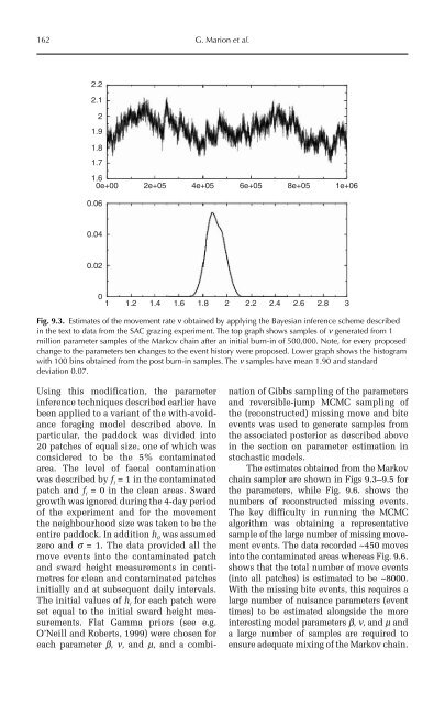
Fig. 9.3. Estimates of the movement rate ν obtained by applying the Bayesian inference scheme described
in the text to data from the SAC grazing experiment. The top graph shows samples of n generated from 1
million parameter samples of the Markov chain after an initial burn-in of 500,000. Note, for every proposed
change to the parameters ten changes to the event history were proposed. Lower graph shows the histogram
with 100 bins obtained from the post burn-in samples. The n samples have mean 1.90 and standard
deviation 0.07.
nation of Gibbs sampling of the parameters
and reversible-jump MCMC sampling of
the (reconstructed) missing move and bite
events was used to generate samples from
the associated posterior as described above
in the section on parameter estimation in
stochastic models.
The estimates obtained from the Markov
chain sampler are shown in Figs 9.3–9.5 for
the parameters, while Fig. 9.6. shows the
numbers of reconstructed missing events.
The key difficulty in running the MCMC
algorithm was obtaining a representative
sample of the large number of missing movement
events. The data recorded ~450 moves
into the contaminated areas whereas Fig. 9.6.
shows that the total number of move events
(into all patches) is estimated to be ~8000.
With the missing bite events, this requires a
large number of nuisance parameters (event
times) to be estimated alongside the more
interesting model parameters b, n, and m and
a large number of samples are required to
ensure adequate mixing of the Markov chain.