- Page 1 and 2:
A cortical model of object percepti
- Page 3 and 4:
A cortical model of object percepti
- Page 6 and 7:
Contents Ab.stract V AcknowlcdRcnie
- Page 8:
4.7 Original contrihutions in this
- Page 11 and 12:
3.9 Example of belief propagation i
- Page 13 and 14:
5.19 SI and CI model responses to a
- Page 15 and 16:
XVI
- Page 17 and 18:
2009 Durabernal S. Wennekers T, Den
- Page 19 and 20:
J.I. OVERVIEW retinal stimulation (
- Page 21 and 22:
J.2. MAIN CONTRfBUTlONS • A revie
- Page 23 and 24:
2,1. OBJECT RECOGNITION ihe princip
- Page 25 and 26:
2.1. OBJECT REC(JGNmON The dorsal s
- Page 27 and 28:
2.1. OBJECT RECOGNJTION properties
- Page 29 and 30:
2.1. OBJECT RECOGNITION of input em
- Page 31 and 32:
2.1. OBJEOTRBCXiGNrnON ta) u I/I ^.
- Page 33 and 34:
2.1. OBJECT RECOGNITION 2.1.2.1 HMA
- Page 35 and 36:
2.1. OBJECT RECnCNmON unit will be
- Page 37 and 38:
2.1. OBJECT REC(X}NIT!ON tivity, st
- Page 39 and 40:
2.1. OBJECT RECOGNITION response fr
- Page 41 and 42:
2.2. HSGH-LEVEL FEEDBACK feature an
- Page 43 and 44:
2.2. HIGH-LEVEL FEEDBACK Thirdly, p
- Page 45 and 46:
2.2. mCH-LBVEL FEEDBACK Kandom 2 LO
- Page 47 and 48:
1.2. HIGH-LEVEL FEEDBACK « 70 U M
- Page 49 and 50:
2.2. HIGH-LEVEL FEEDBACK D Receptiv
- Page 51 and 52:
1.1. HIGH-LEVEL FEEDBACK context of
- Page 53 and 54:
2.2. HIGH-LEVEL FEEDBACK detailed i
- Page 55 and 56:
2.2. HIGH-LEVEL FEEDBACK activity g
- Page 57 and 58:
2.2. HIGH-LEVEL FEEDBACK task, such
- Page 59 and 60:
2.2. HIGH'lM^im,_WEDBACK 2004), and
- Page 61 and 62:
2.2. HIGH-LEVEL FEEDBACK However, t
- Page 63 and 64:
2.2. HIGH-LEVEL FEEDBACK sizes that
- Page 65 and 66:
2.3. ILLUSORY AND OCCLUDED CONTOURS
- Page 67 and 68:
2.3. ILLUSORY AND OCCLUDED CONTOURS
- Page 69 and 70:
2.3. ILLUSORY AND OCCLUDED CONTOURS
- Page 71 and 72:
2.3. ILLUSORY AND OCCLUDED CONTOURS
- Page 73 and 74:
2.3. ILLUSORY AND OCCLUDED CONTOURS
- Page 75 and 76:
2.3. ILLUSORY AND OCCLUDED CONTOURS
- Page 77 and 78:
2.3. ILLUSORY AND OCCLUDED CONTOURS
- Page 79 and 80:
2.3. a.LVSORY AND OCCLUDED CONTnURS
- Page 81 and 82:
2.4. ORIGINAL CONTRIBUTIONS IN THIS
- Page 83 and 84:
3.1. THE BAYBSIAN BRAIN HYPOTHESIS
- Page 85 and 86:
XI. THEBAYESIANBRAINHYPfmBSIS poste
- Page 87 and 88:
3.1. THE BAYESJAN BRAIN HYPOmESIS T
- Page 89 and 90:
3.2. EVIDENCE FROM THE BRAIN ity in
- Page 91 and 92:
3.3. DEFINITION AND MATHEMATlCACPOR
- Page 93 and 94:
3.3. DEFINITION AND MATHEMATICAL FO
- Page 95 and 96:
XX DEFINITION AND MATHEMATICAL FORM
- Page 97 and 98:
.1,3. DEHNITION AND MATHEMATICAL FO
- Page 99 and 100:
3 J. DEFINITION AND MATHEMATICAL FO
- Page 101 and 102:
3.3. DEFINITION AND MATHFMAnCAL FOR
- Page 103 and 104:
.1.3. DERNrnON AmMAnWMATtCAL FORMUL
- Page 105 and 106:
3.3. DEFINITION AND MATHEMATICAL FO
- Page 107 and 108:
3.5. DEFINITION AND MATHEMATICAL FO
- Page 109 and 110:
3.3. DEFINITION AND MATHEMATICAL FO
- Page 111 and 112:
3.3. DEFINITION Am MATHEMATICAL FOR
- Page 113 and 114:
33. DEFINITION AND MATHEMATICAL FOR
- Page 115 and 116: 3.3. OmNmON AND MATHEMATSOALFORMVLA
- Page 117 and 118: 3.3. DEFlNmON AND MATHEMATICAL FORM
- Page 119 and 120: 3 J. DEFINITION AND MATHEMATICAL f-
- Page 121 and 122: 3.3. DEFINITION AND MATHEMATICAL FO
- Page 123 and 124: 3.3. D^JmnON AND MATHEMATICAL F0RMU
- Page 125 and 126: .1.3. DEFI^anON AND MATHFMATICAL FO
- Page 127 and 128: 3.3. DEFINITION AND MATHEMATICAl. F
- Page 129 and 130: 3J. DEFINITION AND MATHEMATICAL FOR
- Page 131 and 132: 3.4. EXISTING MODELS is on models t
- Page 133 and 134: .1.4. EXISTING MODELS Figure J. 10:
- Page 135 and 136: 3.4. EXISTING MODELS the node encod
- Page 137 and 138: 3.4. EXISTING MOOm^ Type of f>raph
- Page 139 and 140: 3.4. EXISTING MODELS The model comp
- Page 141 and 142: X4. EXISTING MODELS ;v 1,1 gi (8>^8
- Page 143 and 144: 3A. EXISTING MODELS proposes a triv
- Page 145 and 146: 3.4. EXISTING MODELS by the higher
- Page 147 and 148: 3.4. EXISTING MODELS aleni lo findi
- Page 149 and 150: 3.4. EXISTING MODELS Model Epshtein
- Page 151 and 152: 3.4. EXISTING MODELS Fristonelal. 2
- Page 153 and 154: 3.4. EXISTING MODELS Oulgoing teedl
- Page 155 and 156: 3.5. ORIGINAL CONTRIBUTIONS IN THIS
- Page 157 and 158: 4.1 HMAX AS A BAYESIAN NETWORK 4.1
- Page 159 and 160: 4.1. HMAX AS A BAYBSIAN NETWORK ini
- Page 161 and 162: 4.1. HMAX AS A BAYESIAN NETWORK fea
- Page 163 and 164: 4.1. HMAX AS A BAYESIAN NETWORK S3
- Page 165: 4.1. HMAX AS A BAYESIAN NETWORK Nod
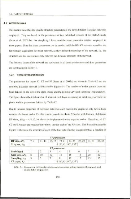
- Page 169 and 170: 4,2. ARCHITECTURES S3 C2 1 node Kj,
- Page 171 and 172: 4.2. ARCmm^TVRES S3 I C2 s f S2 o o
- Page 173 and 174: 4.2. ARCHITECTURES S4 f C3 S3 I C2
- Page 175 and 176: 4.3. LEARNING 4.3.2 S1-C1 CRTs The
- Page 177 and 178: 4.3. LEARNING Weight matrix applied
- Page 179 and 180: 4.3. LEARNING CI group -1 •B •
- Page 181 and 182: 4.3. LEARNING 2. The list of select
- Page 183 and 184: 4.3. LEARNING node=«. Therefore, t
- Page 185 and 186: 4.3. LEARNING 4.3.4 S2-C2CPTS The w
- Page 187 and 188: 4.3. WARNING 60 S3 tealures (object
- Page 189 and 190: 4.4. FEEDFORWARD PROCESSING (he sim
- Page 191 and 192: 4.4. FEEDFORWARD PROCFSSING Figure
- Page 193 and 194: 4.5. FEEDBACK PROCESSING is proport
- Page 195 and 196: 4.5. F^mSACK PRCKESSING n^ (U,) i^(
- Page 197 and 198: 4.5. FEEDBACK PfiOCESSWG t.(VJ,) ji
- Page 199 and 200: 4.5. {REDBACK PROCESSING true vs. r
- Page 201 and 202: 4.5. FEEDBACK PROCES.SING 4.5.3.2 D
- Page 203 and 204: 4.5. FEEDBACK PROCESSING evidence i
- Page 205 and 206: 4.6. SUMMARY OF MODEL APPROXIMATION
- Page 207 and 208: 4.7. ORIGINAL CONTRIBUTIONS IN THIS
- Page 209 and 210: 5,1. FEEDFORWARD PROCESSING using t
- Page 211 and 212: 5.L FEEDFORWARD PROCESSING Slate =
- Page 213 and 214: 5.1. FEEDFORWARD PROCESSING 1^ Onem
- Page 215 and 216: 5.1. FEEDFORWARD PROCESSING j • H
- Page 217 and 218:
5.1. FEEDFORWARD PROCESSING 5.1.2 O
- Page 219 and 220:
5.1. FEEDFORWARD PROCESSING Normal
- Page 221 and 222:
5.1. FEEDFORWARD PROCESSING c g ra
- Page 223 and 224:
5-1. FEEDFORWARD PROCESSING 4 5 Non
- Page 225 and 226:
5.1. FEEDFORWARD PROCESSING 100 8 9
- Page 227 and 228:
S.i. FEEDFORWARD PnOCESSING 5.1.2.4
- Page 229 and 230:
5.2. FEEDBACK-MEDIATED ILLUSORY CON
- Page 231 and 232:
5.2. FEEDBACK MEDIATED ILLUSORY CON
- Page 233 and 234:
5.2. FEiiDBACK-MEDWTHD ILLUSORY CON
- Page 235 and 236:
5.2. FEEDBACK MEDIATED ILLUSORY CON
- Page 237 and 238:
5.2. FEEDBACK-MHDIATED ILLUSORY CON
- Page 239 and 240:
5.2. FEEDBACK'MEDIATED ILLUSORY CON
- Page 241 and 242:
5.2. FEEDBACK-MEDIATED ILLVSORY CON
- Page 243 and 244:
.5.2. FEEDBACK-MEDIATED ELUSORY CON
- Page 245 and 246:
5.2. FEEDBACK-MEDIATED SILUSORY CON
- Page 247 and 248:
5.2. FEEDBACK-MEDIATED ILLUSORY CON
- Page 249 and 250:
5.4. ORIGINAL CONTRIBUTIONS IN THIS
- Page 251 and 252:
6.1. ANALYSIS OF RESULTS dence and
- Page 253 and 254:
6.1. ANALYSIS OF RESULTS The graph
- Page 255 and 256:
6.t. ANALYSIS OF RESULTS used 10 co
- Page 257 and 258:
6.1. ANALYSIS OF RF.SULTS the image
- Page 259 and 260:
6.1. ANALYSIS OF RESULTS feedback w
- Page 261 and 262:
6.1. ANALYSIS OF RESULTS over lime.
- Page 263 and 264:
6.1. ANALYSIS OF RESULTS 6.1.2.5 Fe
- Page 265 and 266:
6.1. ANALYSIS Ot RESULTS step. Alth
- Page 267 and 268:
6.1. ANALYSIS OF RESULTS operations
- Page 269 and 270:
6.J. ANALYSIS OFRBSULTS model could
- Page 271 and 272:
6.1. ANALYSIS OF RESULTS Alternativ
- Page 273 and 274:
6.2. COMPARISON WITH EXPERIMENTAL B
- Page 275 and 276:
6.3. COMPARISON WITH PRKVIOUS MODBL
- Page 277 and 278:
6.4. FUTURE WORK to temporal contex
- Page 279 and 280:
6.5. CONCLUSIONS AND SUMMARY OF CON
- Page 281 and 282:
6.5. CONCLUSIONS AND SUMMARY OF CON
- Page 283 and 284:
• The HTM paliems correspond lo t
- Page 285 and 286:
268
- Page 287 and 288:
270
- Page 289 and 290:
Bolz, J.& Gilbert, CD. (1986), CJcn
- Page 291 and 292:
Friston, K. & Kiebel, S. (2009). 'C
- Page 293 and 294:
Hoffman. K. L. & Lngothetis, N K. (
- Page 295 and 296:
Lanyon. L. & Denham. S. (2(X)9), 'M
- Page 297 and 298:
Murray, M. M.. Wylie. G, R., Higgin
- Page 299 and 300:
Reynolds, J. H. &, Chelazzi, L. (20
- Page 301 and 302:
Stanley. D. A. & Rubin, N. (2003),