reverse engineering – recent advances and applications - OpenLibra

104
Reverse Engineering – Recent Advances and Applications
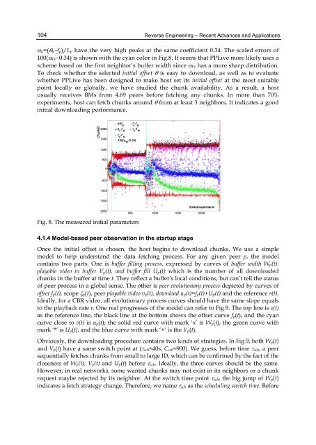
�L=(�h�fp)/Lp have the very high peaks at the same coefficient 0.34. The scaled errors of
100(�W�0.34) is shown with the cyan color in Fig.8. It seems that PPLive more likely uses a
scheme based on the first neighbor’s buffer width since �W has a more sharp distribution.
To check whether the selected initial offset � is easy to download, as well as to evaluate
whether PPLive has been designed to make host set its initial offset at the most suitable
point locally or globally, we have studied the chunk availability. As a result, a host
usually receives BMs from 4.69 peers before fetching any chunks. In more than 70%
experiments, host can fetch chunks around � from at least 3 neighbors. It indicates a good
initial downloading performance.
Fig. 8. The measured initial parameters
4.1.4 Model-based peer observation in the startup stage
Once the initial offset is chosen, the host begins to download chunks. We use a simple
model to help understand the data fetching process. For any given peer p, the model
contains two parts. One is buffer filling process, expressed by curves of buffer width Wp(t),
playable video in buffer Vp(t), and buffer fill Up(t) which is the number of all downloaded
chunks in the buffer at time t. They reflect a buffer’s local conditions, but can’t tell the status
of peer process in a global sense. The other is peer evolutionary process depicted by curves of
offset fp(t), scope �p(t), peer playable video vp(t), download up(t)=fp(t)+Up(t) and the reference s(t).
Ideally, for a CBR video, all evolutionary process curves should have the same slope equals
to the playback rate r. One real progresses of the model can refer to Fig.9. The top line is s(t)
as the reference line, the black line at the bottom shows the offset curve fp(t), and the cyan
curve close to s(t) is up(t); the solid red curve with mark ‘x’ is Wp(t), the green curve with
mark ‘*’ is Up(t), and the blue curve with mark ‘+’ is the Vp(t).
Obviously, the downloading procedure contains two kinds of strategies. In Fig.9, both Wp(t)
and Vp(t) have a same switch point at (�sch≈40s, Csch≈900). We guess, before time �sch, a peer
sequentially fetches chunks from small to large ID, which can be confirmed by the fact of the
closeness of Wp(t), Vp(t) and Up(t) before �sch. Ideally, the three curves should be the same.
However, in real networks, some wanted chunks may not exist in its neighbors or a chunk
request maybe rejected by its neighbor. At the switch time point �sch, the big jump of Wp(t)
indicates a fetch strategy change. Therefore, we name �sch as the scheduling switch time. Before