reverse engineering – recent advances and applications - OpenLibra

More documents

Recommendations

Info

254 Reverse Engineering – Recent Advances and Applications 12 Will-be-set-by-IN-TECH 4.2 Cayley tree model Instead of modeling an acinus as a hierarchical tree of square channels, here we consider these branches as cylinders; this symmetry allows for a continuous description of the concentrations along its branches (Mayo 2009; Mayo et al., 2011). This model is flexible enough to include scaling relationships between parent and daughter branches, giving the total current in terms of the tree’s fractal dimension. 4.2.1 Scaling relationships and fractal dimensions of the fractal Cayley tree To account for scaling between the tree’s branches, we adopt the following labeling scheme. The width and length of each branch is given by 2rei and Lei , respectively, wherein ei = (i, i + 1) label the edges of the Cayley graph in terms of its node, as illustrated by Fig. 5, and i = 0, 1, . . . , n, n + 1, with n being the depth of the tree. The single entrance branch, e0 = (0, 1), is termed the “trunk,” whereas the mn-many terminal branches, each labeled by en = (n, n + 1), are those composing its canopy, or “leaves.” We decompose the tree’s surface into two parts: i) the canopy, or the surface composed of the union of end-caps of the terminal branches, and ii) the tree’s cumulative surface area, or the sum of all surfaces minus the end cross-sections. The width and length of daughter branches can be expressed in terms of the those quantities for the parent branch through scaling relationships for their length, m (Lei )Dtree Dtree = Lei−1 and width, m (rei )Dcanopy Dcanopy = rei−1 (Mandelbrot, 1982). The ratios of these quantities across successive generations can be expressed in terms of the scaling exponents for the cumulative surface of the tree, Dtree , and its canopy, Dcanopy: p = m −1/Dtree , and q = m −1/Dcanopy . (29) For simplicity, we assume the length and width of branches in the same generation are of equal length and width; however, we allow branches to scale in width or length across generations: p = pei = Lei /Lei+1 and q = qei = rei /rei+1 for i = 0, 1, . . . , n − 1. These scaling exponents can be equated with the fractal dimension of the tree’s cumulative and canopy surface areas (Mandelbrot, 1982; Mayo, 2009). 4.2.2 Helmholtz approximation of the full diffusion-reaction problem in a single branch For cylindrical branches in which the ratio of radius to length, termed the aspect ratio, r/L, is “small,” the oxygen concentration is, to very good approximation, dependent only on the variable describing its axis, x (Mayo, 2009). Mass-balance of the oxygen flux in the cylinder gives a Helmholtz-style equation for the concentration in the tube (Mayo et al., 2011): d2 � �2 φ c (x) − c (x) = 0. (30) dx2 L wherein the Thiele modulus of the branch is given in terms of the exploration length: � 2 φ = L . (31) rΛ The tree is composed of three classes of branches, each defined by type of boundary condition given across the beginning and end of the tube. Giving an exit concentration (written in terms
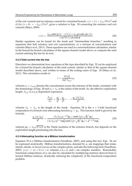
Reverse-Engineering the Robustness of Mammalian Lungs Reverse-Engineering the Robustness of Mammalian Lungs 13 of the exit current) and an entrance current for a terminal branch, c (x = L) = Iext/Wπr 2 and d/dxc (x = 0) = −Ient/Dπr 2 , gives a solution to Eqn. 30 connecting the entrance and exit currents (Mayo, 2009): c (x) = Ient sinh [φ (1 − x/L)]+Iextφ cosh (φx/L) (πρ2 . (32) D/L) φ cosh φ Similar equations can be found for the trunk and “intermediate branches,” resulting in equations that link entrance and exit concentrations, or a mixture of concentrations and currents (Mayo et al., 2011). These equations are used in a renormalization calculation, similar to the branch-by-branch calculation of the square-channel model above, to compute the total current entering the tree by its root. 4.2.3 Total current into the tree Elsewhere we demonstrate how equations of the type described by Eqn. 32 can be employed for a branch-by-branch calculation of the total current, similar to that of the square-channel model described above, and written in terms of the scaling ratios of Eqn. 29 (Mayo et al., 2011). This calculation results in I = Dπr2 0 mq2 c0, (33) Λeff wherein c0 = cent,0 denotes the concentration across the entrance of the trunk, consistent with the terminology of Eqn. 28 and r0 = re0 is the radius of the trunk. So, the effective exploration length, Λeff is a p, q–dependent expression, Λeff L0 = g0 q 2 ◦ g 1 q2 ◦···◦ gn (Λ/L0) q2 , (34) wherein L0 = Le0 is the length of the trunk. Equation 34 is the n + 1–fold functional composition of a branch-wise attenuating function gi = gei . This function itself is given by the formula gi (Λ/L0) q2 (Λ/L0) q = −i/2φ0 + tanh [ � p/ √ q �i φ0] , (35) (Λ/L0) q 2−i mφ 2 0 tanh [� p/ √ q � i φ0]+q 2−i/2 mφ0 √ wherein φ0 = L0 2/r0Λ is the Thiele modulus of the entrance branch, but depends on the exploration length penetrating into the tree. 4.2.4 Attenuating function as a Möbius transformation Equation 35 is a Möbius transformation (Needham, 2007), and using this fact, Eqn. 34 can be expressed analytically. Möbius transformations, denoted by μ, are mappings that rotate, stretch, shrink, or invert curves on the complex plane, and take the following form (Needham, 2007): μ (z) = az + b/cz + d, wherein a, b, c, d, and z are complex numbers. Remarkably, functional compositions of μ can also be calculated by multiplying matrices derived from it, termed Möbius matrices, drastically reducing the complexity of the functional-composition problem. 255
Page 1 and 2:
REVERSE ENGINEERING - RECENT ADVANC
Page 5 and 6:
Contents Preface IX Part 1 Software
Page 9 and 10:
Preface Introduction In the recent
Page 11 and 12:
Preface XI and con’s related to t
Page 13 and 14:
Preface XIII the step-by-step appli
Page 17:
Part 1 Software Reverse Engineering
Page 20 and 21:
4 Reverse Engineering - Recent Adva
Page 22 and 23:
Page 24 and 25:
Page 26 and 27:
10 Reverse Engineering - Recent Adv
Page 28 and 29:
Page 30 and 31:
Page 32 and 33:
Page 34 and 35:
Page 36 and 37:
Page 38 and 39:
Page 40 and 41:
Page 42 and 43:
Page 44 and 45:
Page 46 and 47:
Page 48 and 49:
Page 50 and 51:
Page 52 and 53:
Page 54 and 55:
Page 56 and 57:
Page 58 and 59:
Page 60 and 61:
Page 62 and 63:
Page 64 and 65:
Page 66 and 67:
Page 68 and 69:
Page 70 and 71:
Page 72 and 73:
Page 74 and 75:
58 2. Model driven architecture: An
Page 76 and 77:
Page 78 and 79:
62 Fig. 1. Model, metamodels and tr
Page 80 and 81:
Page 82 and 83:
Page 84 and 85:
Page 86 and 87:
Page 88 and 89:
Page 90 and 91:
Page 92 and 93:
Page 94 and 95:
Page 96 and 97:
Page 98 and 99:
Page 100 and 101:
Page 102 and 103:
Page 104 and 105:
Page 106 and 107:
Page 108 and 109:
Page 110 and 111:
Page 112 and 113:
Page 114 and 115:
Page 116 and 117:
100 Reverse Engineering - Recent Ad
Page 118 and 119:
Page 120 and 121:
Page 122 and 123:
Page 124 and 125:
108 Table 1. Number of smoothers an
Page 126 and 127:
Page 128 and 129:
Page 130 and 131:
Page 133 and 134:
1. Introduction 60 Surface Reconstr
Page 135 and 136:
Surface Reconstruction from Unorgan
Page 137 and 138:
Page 139 and 140:
Page 141 and 142:
Page 143 and 144:
Page 145 and 146:
Page 147 and 148:
Page 149 and 150:
1. Introduction A Systematic Approa
Page 151 and 152:
A Systematic Approach for Geometric
Page 153 and 154:
Page 155 and 156:
Page 157 and 158:
Page 159 and 160:
Page 161 and 162:
Page 163 and 164:
Page 165 and 166:
Page 167 and 168:
Page 169 and 170:
Page 171 and 172:
Page 173 and 174:
Page 175 and 176:
Page 177 and 178:
A Review on Shape Engineering and D
Page 179 and 180:
Page 181 and 182:
Page 183 and 184:
Page 185 and 186:
Page 187 and 188:
Page 189 and 190:
Page 191 and 192:
Page 193 and 194:
Page 195 and 196:
Page 197 and 198:
Page 199 and 200:
Page 201 and 202:
Page 203 and 204:
Integrating Reverse Engineering and
Page 205 and 206:
Page 207 and 208:
Page 209 and 210:
Page 211 and 212:
Page 213 and 214:
Page 215 and 216:
Page 217 and 218:
Page 219 and 220: Integrating Reverse Engineering and
Page 231: Part 3 Reverse Engineering in Medic
Page 234 and 235: 218 Reverse Engineering - Recent Ad
Page 254 and 255: 238 5. Summary and discussions Reve
Page 284 and 285: 268 Fig. 6. A closed polygon mesh r
Page 288 and 289: 272 3. Results Reverse Engineering
Page 292: 276 Reverse Engineering - Recent Ad
show all

reverse engineering – recent advances and applications - OpenLibra

Create successful ePaper yourself

Delete template?

Save as template?