Exámenes resueltos.

More documents

Recommendations

Info

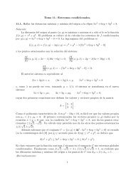
AMPLIACIÓN DE CÁLCULO (Curso 2004/2005) Convocatoria de febrero 15.02.05 PROBLEMA 2 (3 puntos) 1) Calcular el campo escalar u : R 3 −→ R de clase C 1 para que el campo vectorial F definido por: sea conservativo en R 3 . F (x, y, z) = (xy 2 z 2 − 2xy, u(x, y, z), x 2 y 2 z + 1) y F (0, y, z) = (0, y, 1) , 2) En tal caso, calcular la circulación de F sobre la curva Γ definida por las ecuaciones x − z = 0 (xz + yz + y 2 − 3) − √ 1 − x 2 = 0 desde el punto A := (0, 2, 0) hasta el punto B := (1, 1, 1). 3) Calcular la circulación del campo vectorial G definido mediante G(x, y, z) = (y 2 x 2 z − 2yz, x 3 yz − xz + y, x 3 y 2 + 1) sobre el mismo arco de la curva Γ considerado en el apartado anterior. Respuesta: 1) Si F es irrotacional, como el dominio R3 es estrellado, F será conservativo. Imponemos, pues: 0 = −→ i j k rotF = ∂ ∂ ∂ ∂x ∂y ∂z xy2z 2 − 2xy u(x, y, z) x2y2 z + 1 = 2x 2 yz − ∂u ∂u , 0 , ∂z ∂x − 2xyz2 + 2x =⇒ ∂u ∂x = 2xyz2 − 2x =⇒ u = x 2 yz 2 − x 2 + α(y, z) =⇒ 2x 2 yz = ∂u ∂z = 2x2yz + ∂α ∂z luego α(y, z) solo depende de y. Por otra parte, y se tiene (y, z) =⇒ ∂α ∂z F (0, y, z) = (0, y, 1) =⇒ y = u(0, y, z) = α(y, z), u = x 2 yz 2 − x 2 + y. 2) Llamamos L, M, N a las tres componentes de F . Fijado un punto del dominio, por ejemplo, el origen, un potencial escalar U, es decir, un campo que verifica F = −−→ grad U, se puede obtener por la conocida fórmula x y z U(x, y, z) = L(r, 0, 0) dr + M(x, s, 0) ds + N(x, y, t) dt 0 y 0 0 = (−x 2 z + s) ds + (x 2 y 2 t + 1) dt = 0 −x 2 s + s2 s=y 2 s=0 = −x 2 y + y2 2 + x2y2z 2 + z. 2 0 2 2 2 t=z x y t + + t2 2 t=0 = 0,
La circulación que se pide será F · dr = U(1, 1, 1) − U(0, 2, 0) = −1. Γ 3) El campo G no es conservativo pero, en el plano x = z, coincide con F . Por tanto, como Γ está contenida en ese plano, se tiene: G · dr = F · dr = −1. Γ Γ
Page 3 and 4: AMPLIACIÓN DE CÁLCULO (Curso 2001
Page 5 and 6: siendo C una constante arbitraria.
Page 7 and 8: Ω grad( 1 r ) 2 dxdydz y J =
Page 11 and 12: es igual a la integral del campo en
Page 19 and 20: Llamemos C a la circunferencia del
Page 21 and 22: Procederemos parametrizando S ′ e
Page 23 and 24: necesarias anteriores también son
Page 25 and 26: se obtiene Gdr = Γ = S F · nd
Page 31 and 32: de donde se concluye que el flujo d
Page 33 and 34: Calculemos, por tanto, dicha integr
Page 35 and 36: donde el primer límite se calcula
Page 37: z = y (que es π/4) y z = ( √ 2/2
Page 41 and 42: entonces la integral de línea del
Page 43 and 44: de donde, luego (d) Para p > 0, se
Page 45 and 46: Utilizando las propiedades de las f
Page 47 and 48: el centro de gravedad de un triáng
Page 49 and 50: Calculemos I := D (1 − ax − by)
Page 51 and 52: Integremos ∂R/∂x y ∂Q/∂x en
Page 53 and 54: Por tanto, y 0 ψ ϕ B G • Γ A a
Page 57 and 58: • En el caso de la superficie esf
Page 61 and 62: Por tanto, xD = Ix Área = πa√2
Page 65 and 66: 3) Un enunciado del teorema de Stok
Page 67 and 68: 2) El recinto D del enunciado apare
Page 69 and 70: y ∞ 1 La integral γ converge ab
Page 75 and 76: e (3) Para calcular las coordenadas
Page 77 and 78: con lo que el vector normal, que de
Page 79 and 80: 2) Alternativas. El teorema de Gaus
Page 81 and 82: 2. (2 puntos) Determinar los valore
Page 83 and 84: 2) Si representamos el campo F en l
Page 85 and 86: y, por tanto: F · ds = 4MDXg(D) +
Page 87 and 88: 2. Parametrizamos la superficie Σ
Page 89 and 90:
F (a0) converge para algún valor a
Page 91 and 92:
= 1 2π 2 ∗ 2π + 0 + cos 3 0 2
Page 93 and 94:
AMPLIACIÓN DE CÁLCULO (Curso 2006
Page 95 and 96:
Page 97 and 98:
son, por definición, las siguiente
Page 99 and 100:
Page 101 and 102:
Page 103 and 104:
entonces r ′ (t) = (x ′ (t) , y
Page 105 and 106:
Cuando a = 1 la función subintegra
Page 107 and 108:
para a > 0, donde se ha usado que l
Page 109 and 110:
Como = 3a2 2 Por otra parte, la lon
Page 111 and 112:
Page 113 and 114:
lo que desaconseja utilizar este pr
Page 115 and 116:
A continuación se detallan tres po
Page 117 and 118:
Por (a) Ap diverge si p ≤ 0. Adem
Page 119 and 120:
Page 121 and 122:
e integrando: Σ1 F = = t2 2 −
Page 123 and 124:
Se tiene de donde ya que Por otra p
Page 125 and 126:
de modo que x = 0 ⇒ t = − π 2
Page 127 and 128:
Nota 1. El cálculo de x0, que no s
Page 129 and 130:
Para ello existen varias alternativ
Page 131 and 132:
= C [0,2π]×[0, √ 3] 3 − z(r
Page 133 and 134:
2. La superficie Σ está contenida
Page 135 and 136:
Page 137 and 138:
(5) Obtenemos fácilmente resulta
Page 139 and 140:
Apdo. 1. La densidad es ρ(x, y, z)
Page 141 and 142:
y por tanto φ = Σ2 yds = T 1
Page 143 and 144:
Parametrización de Γ2: Ya hemos o
Page 145 and 146:
Page 147 and 148:
y, como lím e k→∞ −k2 = 0, l
Page 149 and 150:
Obsérvese que aunque H es solenoid
Page 151 and 152:
donde se ha usado que Π es un cír
Page 153 and 154:
show all

Exámenes resueltos.

You also want an ePaper? Increase the reach of your titles

Delete template?

Save as template?