Introduction to Stata 8 - (GRIPS

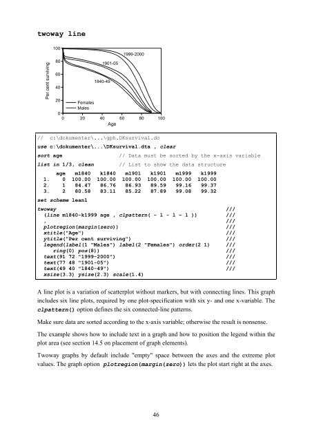
twoway line
Per cent surviving
100
80
60
40
20
0
Females
Males
1901-05
1840-49
1999-2000
0 20 40 60 80 100
Age
/ / c:\dokumenter\...\gph.DKsurvival.do
use
c:\dokumenter\...\DKsurvival.dta , clear
s ort age // Data must be sorted by the x-axis variable
l ist in 1/3, clean // List to show the data structure
age m1840 k1840 m1901 k1901 m1999 k1999
1. 0 100.00 100.00 100.00 100.00 100.00 100.00
2. 1 84.47 86.76 86.93 89.59 99.16 99.37
3. 2 80.58 83.11 85.22 87.89 99.08 99.32
set
scheme lean1
twoway ///
(line m1840-k1999 age , clpattern( - l - l – l )) ///
, ///
plotregion(margin(zero)) ///
xtitle("Age") ///
ytitle("Per cent surviving") ///
legend(label(1 "Males") label(2 "Females") order(2 1) ///
ring(0) pos(8)) ///
text(91 72 "1999-2000") ///
text(77 48 "1901-05") ///
text(49 40 "1840-49") ///
xsize(3.3) ysize(2.3) scale(1.4)
A line plot is a variation of scatterplot without markers, but with connecting lines. This graph
includes six line plots, required by one plot-specification with six y- and one x-variable. The
clpattern() option defines the six connected-line patterns.
Make sure data are sorted according to the x-axis variable; otherwise the result is nonsense.
The example shows how to include text in a graph and how to position the legend within the
plot area (see section 14.5 on placement of graph elements).
Twoway graphs by default include "empty" space between the axes and the extreme plot
values. The graph option plotregion(margin(zero)) lets the plot start right at the axes.
46