Report No xxxx - Instytut Fizyki JÄ drowej PAN

MAGNETIC SUSCEPTIBILITY EVALUATION BY MEANS OF MRI
TECHNIQUE
Ing. Miloslav Steinbauer 1 , Ing. Karel Bartušek, DrSc 2
1 Faculty of Electrical Engineering and Communication, Brno University of Technology,
Purkyňova 464/118, 612 00 Brno, steinbau@feec.vutbr.cz; 2 Institute of Scientific
Instruments, Academy of Sciences of the Czech Republic, Královopolská 147, 612 00 Brno,
bar@isibrno.cz
The determination of magnetic susceptibility of weakly magnetic materials is simple
for substances giving MR signal by comparison with substance, whose susceptibility is
known [2]. In this paper we will discuss measuring technique suitable for substances with no
signal in MR tomography.
This method is based on constant magnetic flux in working space superconducting
magnet. Inserting of the specimen with different value of magnetic susceptibility causes local
deformation of homogeneous magnetic field – idealized example see Fig. 1. Using MRI field
echo technique we can acquire image of the magnetic field homogeneity in measured volume
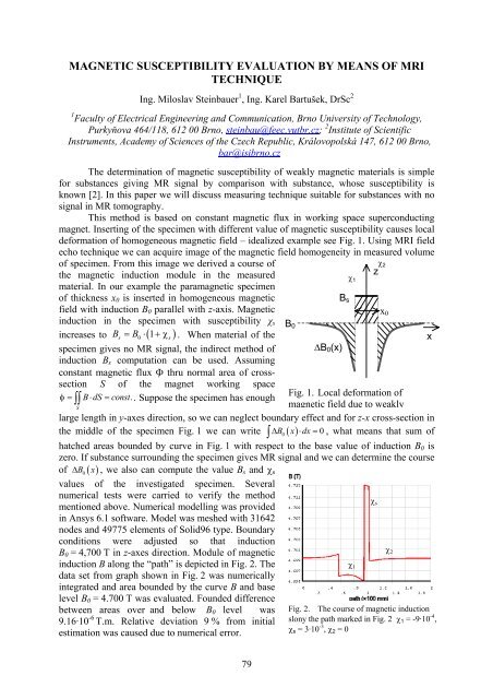
of specimen. From this image we derived a course of
the magnetic induction module in the measured
z χ 2
χ 1
material. In our example the paramagnetic specimen
of thickness x 0 is inserted in homogeneous magnetic
B s
field with induction B 0 parallel with z-axis. Magnetic
x 0
induction in the specimen with susceptibility χ s B 0
increases to Bs
= B0 ⋅ ( 1+
χs)
. When material of the
x
specimen gives no MR signal, the indirect method of ∆B 0 (x)
induction Bs computation can be used. Assuming
constant magnetic flux Φ thru normal area of crosssection
S of the magnet working space
φ = B ⋅dS
=const.
Fig. 1. Local deformation of
∫∫
. Suppose the specimen has enough
S
magnetic field due to weakly
large length in y-axes direction, so we can neglect boundary effect and for z-x cross-section in
the middle of the specimen Fig. 1 we can write ∫ ∆ B0 ( x)
⋅ dx = 0 , what means that sum of
hatched areas bounded by curve in Fig. 1 with respect to the base value of induction B0 is
zero. If substance surrounding the specimen gives MR signal and we can determine the course
of ∆B0
( x)
, we also can compute the value B s and χ s
values of the investigated specimen. Several
numerical tests were carried to verify the method
χ s
mentioned above. Numerical modelling was provided
in Ansys 6.1 software. Model was meshed with 31642
nodes and 49775 elements of Solid96 type. Boundary
conditions were adjusted so that induction
B 0 = 4,700 T in z-axes direction. Module of magnetic
χ 2
induction B along the “path” is depicted in Fig. 2. The
χ 1
data set from graph shown in Fig. 2 was numerically
integrated and area bounded by the curve B and base
level B 0 = 4.700 T was evaluated. Founded difference
between areas over and below B 0 level was Fig. 2. The course of magnetic induction
9.16·10 -6 T.m. Relative deviation 9 % from initial slony the path marked in Fig. 2 χ 1 = -9·10 -4 ,
estimation was caused due to numerical error.
χ s = 3·10 -3 , χ 2 = 0
79