- Page 2:
Reservoir Geomechanics This interdi
- Page 8:
cambridge university press Cambridg
- Page 14:
Contents Preface page xi PART I: BA
- Page 18:
ix Contents More on drilling-induce
- Page 22:
Preface This book has its origin in
- Page 26:
xiii Preface done with Pavel Peska
- Page 34:
1 The tectonic stress field My goal
- Page 38:
5 The tectonic stress field chapter
- Page 42:
7 The tectonic stress field signifi
- Page 46:
9 The tectonic stress field S v Nor
- Page 50:
0 SEAFLOOR 2000 Depth (feet below s
- Page 54:
a. Stress or pressure 0 20 40 60 80
- Page 58:
15 The tectonic stress field The o
- Page 62:
17 The tectonic stress field Observ
- Page 66:
180˚ 216˚ 252˚ 288˚ 324˚ 64˚
- Page 70:
21 The tectonic stress field 121 o
- Page 74:
23 The tectonic stress field 62N 0
- Page 78: a. Margarita Pays b. Stress state a
- Page 82: 2 Pore pressure at depth in sedimen
- Page 86: 29 Pore pressure at depth in sedime
- Page 90: 31 Pore pressure at depth in sedime
- Page 94: 33 Pore pressure at depth in sedime
- Page 98: 35 Pore pressure at depth in sedime
- Page 102: 37 Pore pressure at depth in sedime
- Page 106: 39 Pore pressure at depth in sedime
- Page 110: 41 Pore pressure at depth in sedime
- Page 114: 43 Pore pressure at depth in sedime
- Page 118: 45 Pore pressure at depth in sedime
- Page 122: 47 Pore pressure at depth in sedime
- Page 126: a. 2000 OFFSHORE TRINIDAD CENTER OF
- Page 132: a. W Shot Number E 1300 1400 1500 1
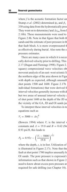
- Page 136: a. f BURIAL AT HYDROSTATIC Porosity
- Page 140: 3 Basic constitutive laws 56 In thi
- Page 144: Stress (MPa) 58 Reservoir geomechan
- Page 148: 60 Reservoir geomechanics Figure 3.
- Page 152: 62 Reservoir geomechanics 10 SANDST
- Page 156: 64 Reservoir geomechanics Table 3.1
- Page 160: 66 Reservoir geomechanics Biot (196
- Page 164: 68 Reservoir geomechanics for very
- Page 168: a. 10 8 DYNAMIC MODULI (ULTRASONIC)
- Page 172: 72 Reservoir geomechanics in veloci
- Page 176: 74 Reservoir geomechanics a. b. Ins
- Page 180:
76 Reservoir geomechanics such that
- Page 184:
78 Reservoir geomechanics Mechanica
- Page 188:
80 Reservoir geomechanics of the hi
- Page 192:
82 Reservoir geomechanics The total
- Page 196:
4 Rock failure in compression, tens
- Page 200:
S 3 S 1 86 Reservoir geomechanics S
- Page 204:
a. s 1 b s n t s 3 b. t Mohr envelo
- Page 208:
90 Reservoir geomechanics a. Shear
- Page 212:
92 Reservoir geomechanics STRONG RO
- Page 216:
94 Reservoir geomechanics 150 s 3 1
- Page 220:
96 Reservoir geomechanics a. b. 125
- Page 224:
98 Reservoir geomechanics a. 300 25
- Page 228:
100 Reservoir geomechanics p a is a
- Page 232:
102 Reservoir geomechanics Drucker-
- Page 236:
104 Reservoir geomechanics wellbore
- Page 240:
106 Reservoir geomechanics b. t m 0
- Page 244:
108 Reservoir geomechanics a. 300 M
- Page 248:
a. 300 6000 4000 3000 V p (m/s) 200
- Page 252:
a. 300 250 5000 21 4000 V p (m/s) 3
- Page 256:
114 Reservoir geomechanics Table 4.
- Page 260:
116 Reservoir geomechanics Table 4.
- Page 264:
118 Reservoir geomechanics velocity
- Page 268:
120 Reservoir geomechanics 300 S v
- Page 272:
122 Reservoir geomechanics 300 250
- Page 276:
124 Reservoir geomechanics Because
- Page 280:
126 Reservoir geomechanics Maximum
- Page 284:
128 Reservoir geomechanics S 1 - S
- Page 288:
130 Reservoir geomechanics Healy (1
- Page 292:
132 Reservoir geomechanics fault (t
- Page 296:
a. Stress or pressure 0 20 40 60 80
- Page 300:
136 Reservoir geomechanics m i Shea
- Page 304:
138 Reservoir geomechanics a. SHmax
- Page 308:
5 Faults and fractures at depth 140
- Page 312:
142 Reservoir geomechanics S Hmax
- Page 316:
a. JOINT SHEARED JOINT ONSET OF DAM
- Page 320:
146 Reservoir geomechanics Wellbore
- Page 324:
Depth (feet) 148 Reservoir geomecha
- Page 328:
150 Reservoir geomechanics UP (DIP
- Page 332:
152 Reservoir geomechanics a. 6500
- Page 336:
154 Reservoir geomechanics in Figur
- Page 340:
156 Reservoir geomechanics Alternat
- Page 344:
158 Reservoir geomechanics a. N b.
- Page 348:
160 Reservoir geomechanics a. Doubl
- Page 352:
162 Reservoir geomechanics A D B C
- Page 358:
Part II Measuring stress orientatio
- Page 364:
168 Reservoir geomechanics stress c
- Page 368:
170 Reservoir geomechanics trajecto
- Page 372:
172 Reservoir geomechanics strongly
- Page 376:
174 Reservoir geomechanics boundary
- Page 380:
a. b. N E S W N N E S W N c. 0 W BO
- Page 384:
178 Reservoir geomechanics In Figur
- Page 388:
180 Reservoir geomechanics a. A S H
- Page 392:
182 Reservoir geomechanics a. 10 12
- Page 396:
184 Reservoir geomechanics X-STRUCT
- Page 400:
186 Reservoir geomechanics a. 150 1
- Page 404:
188 Reservoir geomechanics stress-i
- Page 408:
190 Reservoir geomechanics and then
- Page 412:
192 Reservoir geomechanics a. 180 7
- Page 416:
194 Reservoir geomechanics a. 150 s
- Page 420:
196 Reservoir geomechanics More on
- Page 424:
198 Reservoir geomechanics with tim
- Page 428:
200 Reservoir geomechanics a. b. Fi
- Page 432:
202 Reservoir geomechanics virtual
- Page 436:
204 Reservoir geomechanics Table 6.
- Page 440:
7 Determination of S 3 from mini-fr
- Page 444:
208 Reservoir geomechanics stress o
- Page 448:
210 Reservoir geomechanics The othe
- Page 452:
212 Reservoir geomechanics supplies
- Page 456:
214 Reservoir geomechanics 0 0 Stre
- Page 460:
216 Reservoir geomechanics a. 8 7 P
- Page 464:
218 Reservoir geomechanics a. -400
- Page 468:
220 Reservoir geomechanics Can hydr
- Page 472:
222 Reservoir geomechanics the hydr
- Page 476:
224 Reservoir geomechanics a. b. 15
- Page 480:
226 Reservoir geomechanics 138 124
- Page 484:
228 Reservoir geomechanics used var
- Page 488:
230 Reservoir geomechanics 0 1000 2
- Page 492:
232 Reservoir geomechanics 5390 Bre
- Page 496:
234 Reservoir geomechanics and Zoba
- Page 500:
236 Reservoir geomechanics the prin
- Page 504:
238 Reservoir geomechanics are give
- Page 508:
240 Reservoir geomechanics a. b. c.
- Page 512:
242 Reservoir geomechanics discusse
- Page 516:
244 Reservoir geomechanics a. b. Te
- Page 520:
246 Reservoir geomechanics a. s min
- Page 524:
248 Reservoir geomechanics b. Botto
- Page 528:
250 Reservoir geomechanics 80 25 MP
- Page 532:
252 Reservoir geomechanics a. 180 b
- Page 536:
254 Reservoir geomechanics a. b. c.
- Page 540:
256 Reservoir geomechanics ∼1-5 k
- Page 544:
258 Reservoir geomechanics a. b. S
- Page 548:
260 Reservoir geomechanics a. Boreh
- Page 552:
262 Reservoir geomechanics True fas
- Page 556:
264 Reservoir geomechanics Figure 8
- Page 560:
9 Stress fields - from tectonic pla
- Page 564:
180˚ 270˚ 0˚ 90˚ 180˚ 70˚ 70
- Page 568:
270 Reservoir geomechanics subjecte
- Page 572:
1 1 9 o E 8 o E 7 o E 6 o E 5 o E 4
- Page 576:
274 Reservoir geomechanics a. b. 62
- Page 580:
276 Reservoir geomechanics 7000 Nor
- Page 584:
a. 8000 Normal faulting Measured S
- Page 588:
280 Reservoir geomechanics Methods
- Page 592:
282 Reservoir geomechanics from 0.4
- Page 596:
284 Reservoir geomechanics the meas
- Page 600:
286 Reservoir geomechanics 0 Equiva
- Page 604:
288 Reservoir geomechanics a. 0 500
- Page 608:
290 Reservoir geomechanics a. b. S
- Page 612:
292 Reservoir geomechanics A few mo
- Page 616:
294 Reservoir geomechanics Pressure
- Page 620:
296 Reservoir geomechanics a. b. 50
- Page 626:
Part III Applications
- Page 632:
302 Reservoir geomechanics The next
- Page 636:
304 Reservoir geomechanics a. Stabl
- Page 640:
306 Reservoir geomechanics to remed
- Page 644:
308 Reservoir geomechanics a. b. c.
- Page 648:
Depth (feet) 310 Reservoir geomecha
- Page 652:
312 Reservoir geomechanics The pred
- Page 656:
314 Reservoir geomechanics a. 13.22
- Page 660:
316 Reservoir geomechanics a. b. 70
- Page 664:
318 Reservoir geomechanics a. N b.
- Page 668:
320 Reservoir geomechanics S Hmax A
- Page 672:
322 Reservoir geomechanics to the a
- Page 676:
324 Reservoir geomechanics and S hm
- Page 680:
326 Reservoir geomechanics 4 P grow
- Page 684:
328 Reservoir geomechanics p w = s
- Page 688:
330 Reservoir geomechanics Figure 1
- Page 692:
332 Reservoir geomechanics Figure 1
- Page 696:
334 Reservoir geomechanics Figure 1
- Page 700:
336 Reservoir geomechanics Figure 1
- Page 704:
338 Reservoir geomechanics Figure 1
- Page 708:
11 Critically stressed faults and f
- Page 712:
342 Reservoir geomechanics a. 0.4 m
- Page 716:
344 Reservoir geomechanics 40 35 30
- Page 720:
346 Reservoir geomechanics with fau
- Page 724:
348 Reservoir geomechanics a. 3000
- Page 728:
Table 11.1. Detection of permeable
- Page 732:
352 Reservoir geomechanics All Plan
- Page 736:
a. ALL FRACTURES FROM SIT FRACTURES
- Page 740:
356 Reservoir geomechanics exploita
- Page 744:
358 Reservoir geomechanics expected
- Page 748:
360 Reservoir geomechanics hole, Sh
- Page 752:
362 Reservoir geomechanics rock wit
- Page 756:
364 Reservoir geomechanics a. A S H
- Page 760:
366 Reservoir geomechanics N EXTENT
- Page 764:
368 Reservoir geomechanics a. A b.
- Page 768:
370 Reservoir geomechanics FILL TO
- Page 772:
372 Reservoir geomechanics Schemati
- Page 776:
374 Reservoir geomechanics Figure 1
- Page 780:
376 Reservoir geomechanics HIGH a.
- Page 784:
12 Effects of reservoir depletion A
- Page 788:
380 Reservoir geomechanics Figure 1
- Page 792:
382 Reservoir geomechanics Figure 1
- Page 796:
384 Reservoir geomechanics There ar
- Page 800:
386 Reservoir geomechanics
- Page 804:
388 Reservoir geomechanics Figure 1
- Page 808:
390 Reservoir geomechanics Zoback a
- Page 812:
392 Reservoir geomechanics Figure 1
- Page 816:
394 Reservoir geomechanics Figure 1
- Page 820:
396 Reservoir geomechanics can also
- Page 824:
398 Reservoir geomechanics and ther
- Page 828:
400 Reservoir geomechanics curve is
- Page 832:
402 Reservoir geomechanics Figure 1
- Page 836:
404 Reservoir geomechanics
- Page 840:
406 Reservoir geomechanics To deter
- Page 844:
408 Reservoir geomechanics Figure 1
- Page 848:
410 Reservoir geomechanics Figure 1
- Page 852:
412 Reservoir geomechanics Hagin an
- Page 856:
414 Reservoir geomechanics Figure 1
- Page 860:
Figure 12.18. (a) Map of southern L
- Page 864:
418 Reservoir geomechanics along a
- Page 868:
420 Reservoir geomechanics Figure 1
- Page 874:
References Aadnoy, B. S. (1990a).
- Page 878:
425 References Bourbie, T., Coussy,
- Page 882:
427 References Coulomb, C. A. (1773
- Page 886:
429 References Flemings, P. B., Stu
- Page 890:
431 References Hayashi, K. and Haim
- Page 894:
433 References Lade, P. (1977). “
- Page 898:
435 References Moos, D. and Zoback,
- Page 902:
437 References Raaen, A. M. and Bru
- Page 906:
439 References Tang, X. M. and Chen
- Page 910:
441 References Wiprut, D. and Zobac
- Page 914:
443 References Zoback, M. L. and a.
- Page 920:
446 Index critically stressed fault
- Page 924:
448 Index ridge push 270 RMS (root
- Page 934:
180˚ 216˚ 252˚ 288˚ 324˚ 64˚
- Page 938:
a. 70 Pressure history - Lapeyrouse
- Page 942:
. 140 a. 120 100 S hmin S Hmax R S
- Page 946:
Figure 6.4. (a) Wellbore breakouts
- Page 950:
a. A S Hmax A-CENTRAL FAULT HIGH RE
- Page 954:
a. b. Figure 6.17. The area in whic
- Page 958:
160 155 150 145 S Hmax (MPa) 140 13
- Page 962:
a. b. Tendency for breakouts Orient
- Page 966:
180˚ 270˚ 0˚ 90˚ 180˚ 70˚ 70
- Page 970:
Depth (feet) S Hmax N S hmin W S v
- Page 974:
Figure 10.9. (a) Probability densit
- Page 978:
S Hmax ABOVE THE FAULT 9 10 11 12 R
- Page 982:
-9 200' - 9200 ' - 9 600 ' a. LESS
- Page 986:
a. 0.4 m = 1.0 m = 0.6 t/S v 0.2 0
- Page 990:
a. 3000 S Hmax = 10N 3100 3200 Dept
- Page 994:
a. ALL FRACTURES FROM SIT FRACTURES
- Page 998:
a. A S Hmax A-CENTRAL FAULT HIGH RE
- Page 1002:
a. A b. N N A B C B C D D E E 0 1 2
- Page 1006:
N Vertical Displacement cm 2 N East