- Page 1 and 2: POLITECHNIKA WARSZAWSKA WARSAW UNIV
- Page 3 and 4: Contents 1. Introduction 4 2. Mathe
- Page 5 and 6: 1. Introduction 1. INTRODUCTION The
- Page 7 and 8: 1. Introduction In the author’s o
- Page 9 and 10: 2. Mathematical description of indu
- Page 11 and 12: 2. Mathematical description of indu
- Page 13 and 14: 2. Mathematical description of indu
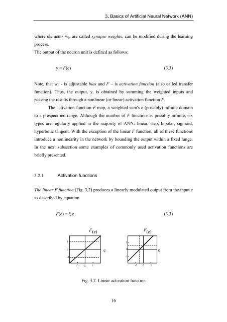
- Page 15: 3. Basics of Artificial Neural Netw
- Page 19 and 20: 3. Basics of Artificial Neural Netw
- Page 21 and 22: 3. Basics of Artificial Neural Netw
- Page 23 and 24: 3. Basics of Artificial Neural Netw
- Page 25 and 26: 3. Basics of Artificial Neural Netw
- Page 27 and 28: 3. Basics of Artificial Neural Netw
- Page 29 and 30: 3. Basics of Artificial Neural Netw
- Page 31 and 32: 3. Basics of Artificial Neural Netw
- Page 33 and 34: 3. Basics of Artificial Neural Netw
- Page 35 and 36: 3. Basics of Artificial Neural Netw
- Page 37 and 38: 3. Basics of Artificial Neural Netw
- Page 39 and 40: 3. Basics of Artificial Neural Netw
- Page 41 and 42: 4. ANN based Current Controllers (C
- Page 43 and 44: 4. ANN based Current Controllers (C
- Page 45 and 46: 4. ANN based Current Controllers (C
- Page 47 and 48: 4. ANN based Current Controllers (C
- Page 49 and 50: 4. ANN based Current Controllers (C
- Page 51 and 52: 4. ANN based Current Controllers (C
- Page 53 and 54: 4. ANN based Current Controllers (C
- Page 55 and 56: 4. ANN based Current Controllers 4.
- Page 57 and 58: 4. ANN based Current Controllers Ta
- Page 59 and 60: 4. ANN based Current Controllers Ta
- Page 61 and 62: 4. ANN based Current Controllers Ta
- Page 63 and 64: 4. ANN based Current Controllers Th
- Page 65 and 66: 4. ANN based Current Controllers As
- Page 67 and 68:
4. ANN based Current Controllers Fi
- Page 69 and 70:
4. ANN based Current Controllers Fi
- Page 71 and 72:
4. ANN based Current Controllers Fi
- Page 73 and 74:
4. ANN based Current Controllers Fi
- Page 75 and 76:
4. ANN based Current Controllers Fi
- Page 77 and 78:
4. ANN based Current Controllers Fi
- Page 79 and 80:
4. ANN based Current Controllers Fi
- Page 81 and 82:
4. ANN based Current Controllers a)
- Page 83 and 84:
4. ANN based Current Controllers th
- Page 85 and 86:
4. ANN based Current Controllers a)
- Page 87 and 88:
4. ANN based Current Controllers an
- Page 89 and 90:
4. ANN based Current Controllers Fi
- Page 91 and 92:
4. ANN based Current Controllers Th
- Page 93 and 94:
4. ANN based Current Controllers Fi
- Page 95 and 96:
4. ANN based Current Controllers Fi
- Page 97 and 98:
4. ANN based Current Controllers Fi
- Page 99 and 100:
5. Speed estimation of induction mo
- Page 101 and 102:
5. Speed estimation of induction mo
- Page 103 and 104:
5. Speed estimation of induction mo
- Page 105 and 106:
5. Speed estimation of induction mo
- Page 107 and 108:
5. Speed estimation of induction mo
- Page 109 and 110:
5. Speed estimation of induction mo
- Page 111 and 112:
5. Speed estimation of induction mo
- Page 113 and 114:
5. Speed estimation of induction mo
- Page 115 and 116:
5. Speed estimation of induction mo
- Page 117 and 118:
5.3.1.2. Improved method based on t
- Page 119 and 120:
Therefore, the discrete model of st
- Page 121 and 122:
6. ANN sensorless Field Oriented Co
- Page 123 and 124:
6. ANN sensorless Field Oriented Co
- Page 125 and 126:
6. ANN sensorless Field Oriented Co
- Page 127 and 128:
6. ANN sensorless Field Oriented Co
- Page 129 and 130:
6. ANN sensorless Field Oriented Co
- Page 131 and 132:
6. ANN sensorless Field Oriented Co
- Page 133 and 134:
6. ANN sensorless Field Oriented Co
- Page 135 and 136:
6. ANN sensorless Field Oriented Co
- Page 137 and 138:
6. ANN sensorless Field Oriented Co
- Page 139 and 140:
6. ANN sensorless Field Oriented Co
- Page 141 and 142:
6. ANN sensorless Field Oriented Co
- Page 143 and 144:
6. ANN sensorless Field Oriented Co
- Page 145 and 146:
6. ANN sensorless Field Oriented Co
- Page 147 and 148:
7. Simulation and experimental resu
- Page 149 and 150:
7. Simulation and experimental resu
- Page 151 and 152:
7. Simulation and experimental resu
- Page 153 and 154:
7. Simulation and experimental resu
- Page 155 and 156:
7. Simulation and experimental resu
- Page 157 and 158:
7. Simulation and experimental resu
- Page 159 and 160:
7. Simulation and experimental resu
- Page 161 and 162:
7. Simulation and experimental resu
- Page 163 and 164:
7. Simulation and experimental resu
- Page 165 and 166:
7. Simulation and experimental resu
- Page 167 and 168:
7. Simulation and experimental resu
- Page 169 and 170:
8. Conclusions 8. CONCLUSIONS The r
- Page 171 and 172:
References REFERENCES Books and Ove
- Page 173 and 174:
References [34] D. Schauder, and R.
- Page 175 and 176:
References [66] A. Tripathi and P.
- Page 177 and 178:
References [97] J. W. Kolar, H. Ert
- Page 179 and 180:
References [129] M. P. Kazmierkowsk
- Page 181 and 182:
A1. Description of the simulation p
- Page 183 and 184:
A1. Description of the simulation p
- Page 185 and 186:
A1. Description of the simulation p
- Page 187 and 188:
A1. Description of the simulation p
- Page 189 and 190:
A1. Description of the simulation p
- Page 191 and 192:
A1. Description of the simulation p
- Page 193 and 194:
A1. Description of the simulation p
- Page 195 and 196:
A2. Laboratory setup A2. Laboratory
- Page 197 and 198:
A2. Laboratory setup A2.3. dSpace D
- Page 199 and 200:
A2. Laboratory setup Offset calibra
- Page 201 and 202:
A2. Laboratory setup consists of an
- Page 203 and 204:
A3. Motor parameters A3. MOTOR PARA
- Page 205 and 206:
A4. Notation - u s - stator voltage


![[TCP] Opis układu - Instytut Sterowania i Elektroniki Przemysłowej ...](https://img.yumpu.com/23535443/1/184x260/tcp-opis-ukladu-instytut-sterowania-i-elektroniki-przemyslowej-.jpg?quality=85)