FOUNDATIONS OF QUANTUM MECHANICS

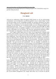
132 CHAPTER VI. BOHMIAN MECHANICS
With
S(⃗q) =
⎧
⎪⎨
⎪⎩
S A (⃗q) for ⃗q ∈ A,
S B (⃗q) for ⃗q ∈ B,
0 elsewhere,
(VI. 17)
and ψ A (⃗q) = R A (⃗q)e i S A(⃗q) , etc., (VI. 14) reads
ψ(⃗q) = ( a R A (⃗q) + b R B (⃗q) ) e i S(⃗q) , (VI. 18)
which means that also the quantum potential, as depicted in figure VI. 1, can now be taken as a sum
of terms belonging to separate areas. The particles in area A do not perceive the wave function in
area B at all.
Figure VI. 2: A simulation of the double slit experiment in Bohmian mechanics. Each particle follows
a certain path between the slits and the photographic plate. All particles coming from the upper slit
arrive at the upper half of the photographic plate, likewise for the lower slit and lower half of the
plate. The twists in the paths are caused by the quantum potential U. (Vigier et al. 1987 )
VI. 3
COMPOSITE SYSTEMS
The technique used to rewrite the Schrödinger equation into equations describing particles with
definite position and momentum in a non - classical potential field, can easily be generalized. For