Subsampling estimates of the Lasso distribution.
Subsampling estimates of the Lasso distribution.
Subsampling estimates of the Lasso distribution.
You also want an ePaper? Increase the reach of your titles
YUMPU automatically turns print PDFs into web optimized ePapers that Google loves.
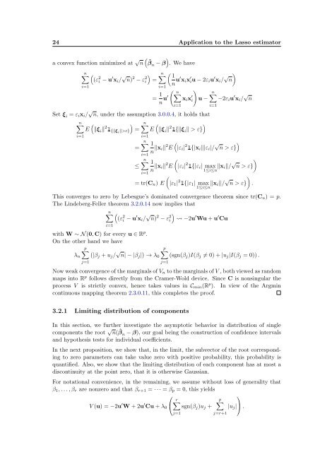
24 Application to <strong>the</strong> <strong>Lasso</strong> estimator<br />
a convex function minimized at √ ( )<br />
n ˆβ n − β . We have<br />
n∑<br />
i=1<br />
(<br />
(ε 2 i − u ′ x i / √ )<br />
n) 2 − ε 2 i =<br />
n∑<br />
( 1<br />
n u′ x i x ′ iu − 2ε i u ′ x i / √ n)<br />
i=1<br />
= 1 ( n<br />
)<br />
∑<br />
n∑<br />
n u′ x i x ′ i u − −2ε i u ′ x i / √ n<br />
i=1<br />
i=1<br />
Set ξ i = ε i x i / √ n, under <strong>the</strong> assumption 3.0.0.4, it holds that<br />
n∑<br />
i=1<br />
(<br />
)<br />
E ‖ξ i ‖ 2 1 {‖ξi ‖>ε} =<br />
=<br />
≤<br />
n∑<br />
i=1<br />
n∑<br />
i=1<br />
n∑<br />
i=1<br />
(<br />
)<br />
E ‖ξ i ‖ 2 1{‖ξ i ‖ > ε}<br />
1 (<br />
n ‖x i‖ 2 E |ε i | 2 1{|x i ‖|ε i |/ √ )<br />
n > ε}<br />
1<br />
n ‖x i‖ 2 E<br />
= tr(C n ) E<br />
(<br />
|ε i | 2 1{|ε i | max ‖x i‖/ √ )<br />
n > ε}<br />
1≤i≤n<br />
(<br />
|ε 1 | 2 1{|ε 1 | max<br />
1≤i≤n ‖x i||/ √ n > ε}<br />
This converges to zero by Lebesgue’s dominated convergence <strong>the</strong>orem since tr(C n ) = p.<br />
The Lindeberg-Feller <strong>the</strong>orem 3.2.0.14 now implies that<br />
n∑<br />
i=1<br />
(<br />
(ε 2 i − u ′ x i / √ )<br />
n) 2 − ε 2 i −2u ′ Wu + u ′ Cu<br />
with W ∼ N (0, C) for every u ∈ R p .<br />
On <strong>the</strong> o<strong>the</strong>r hand we have<br />
p∑ ( |βj + u j / √ n| − |β j | ) p∑<br />
→ λ 0 (sgn(β j )I(β j ≠ 0) + |u j |I(β j = 0)) .<br />
λ n<br />
j=1<br />
j=1<br />
Now weak convergence <strong>of</strong> <strong>the</strong> marginals <strong>of</strong> V n to <strong>the</strong> marginals <strong>of</strong> V , both viewed as random<br />
maps into R p follows directly from <strong>the</strong> Cramer-Wold device. Since C is nonsingular <strong>the</strong><br />
process V is strictly convex, hence takes values in C min (R p ). In view <strong>of</strong> <strong>the</strong> Argmin<br />
continuous mapping <strong>the</strong>orem 2.3.0.11, this completes <strong>the</strong> pro<strong>of</strong>.<br />
)<br />
.<br />
3.2.1 Limiting <strong>distribution</strong> <strong>of</strong> components<br />
In this section, we fur<strong>the</strong>r investigate <strong>the</strong> asymptotic behavior in <strong>distribution</strong> <strong>of</strong> single<br />
components <strong>the</strong> root √ n( ˆβ n − β), our goal being <strong>the</strong> construction <strong>of</strong> confidence intervals<br />
and hypo<strong>the</strong>sis tests for individual coefficients.<br />
In <strong>the</strong> next proposition, we show that, in <strong>the</strong> limit, <strong>the</strong> subvector <strong>of</strong> <strong>the</strong> root corresponding<br />
to zero parameters can take value zero with positive probability, this probability is<br />
quantified. Also, we show that <strong>the</strong> limiting <strong>distribution</strong> <strong>of</strong> each component has at most a<br />
discontinuity at <strong>the</strong> point zero, that it is o<strong>the</strong>rwise Gaussian.<br />
For notational convenience, in <strong>the</strong> remaining, we assume without loss <strong>of</strong> generality that<br />
β 1 , . . . , β r are nonzero and that β r+1 = · · · = β p = 0, this yields<br />
⎛<br />
⎞<br />
r∑<br />
p∑<br />
V (u) = −2u ′ W + 2u ′ Cu + λ 0 ⎝ sgn(β j )u j + |u j | ⎠ .<br />
j=1<br />
j=r+1


