Subsampling estimates of the Lasso distribution.

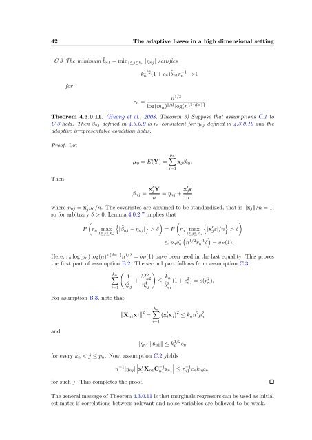
42 The adaptive Lasso in a high dimensional setting
C.3 The minimum ˜b n1 = min 1≤j≤kn |η nj | satisfies
for
r n =
kn
1/2 (1 + c n )˜b n1 rn −1 → 0
n 1/2
log(m n ) 1/d log(n) 1{d=1}
Theorem 4.3.0.11. (Huang et al., 2008, Theorem 3) Suppose that assumptions C.1 to
C.3 hold. Then β nj defined in 4.3.0.9 is r n consistent for η nj defined in 4.3.0.10 and the
adaptive irrepresentable condition holds.
Proof. Let
Then
µ 0 = E(Y) =
˜β nj = x′ j Y
n
p n
∑
j=1
x j β 0j .
= η nj + x′ j ε
n
where η nj = x ′ j µ 0/n. The covariates are assumed to be standardized, that is ‖x j ‖/n = 1,
so for arbitrary δ > 0, Lemma 4.0.2.7 implies that
( {
P r n max | ˜β
} ) ( { } )
nj − η nj | > δ = P r n max |x ′ jε|/n > δ
1≤j≤k n 1≤j≤k n
( )
≤ p n qn
∗ n 1/2 rn
−1 δ = o P (1).
Here, r n log(p n ) log(n) 1{d=1} n 1/2 = o P (1) have been used in the last equality. This proves
the first part of assumption B.2. The second part follows from assumption C.3:
(
∑k n 1
j=1
For asumption B.3, note that
η 2 nj
+ M 2 n2
η 4 nj
)
≤ k n
˜b2 nj
(1 + c 2 n) = o(r 2 n).
and
∥
∥X ′ ∥
n1x j 2 ∑k n
( = x
′ ) 2
i x j ≤ kn n 2 ρ 2 n
i=1
|η nj |‖s n1 ‖ ≤ kn
1/2 c n
for every k n < j ≤ p n . Now, assumption C.2 yields
n −1 ∣
|η nj | ∣x ′ jX n1 C −1
n1 s n1∣ ≤ τn1 −1 c nk n ρ n .
for such j. This completes the proof.
The general message of Theorem 4.3.0.11 is that marginals regressors can be used as initial
estimates if correlations between relevant and noise variables are believed to be weak.