Impact of fuel supply impedance and fuel staging on gas turbine ...

More documents

Recommendations

Info

Numerical simulation area, which is shown in Fig. 6.25. Although the total flame surface is reduced the overall heat release rate increases in the beginning due to the strong increased release <strong>of</strong> heat per unit mass <strong>of</strong> premixture <strong>and</strong> the increased burning velocity. However, once the additional <strong>fuel</strong> injected by the impulse forcing is consumed, the equivalence ratio returns along with ∆H <strong>and</strong> s t to its original value. As the flame surface is still smaller compared to the undisturbed case, ˙Q ′ decreases <strong>and</strong> attains finally negative values. With the burning velocity s t restored to its original value, the flame surface area is now too small to burn the arriving fresh premixture. The flame is thus convected downstream to its original area <strong>and</strong> position. In summary, the overall shape <strong>of</strong> UIR φ <strong>and</strong> in particular the undershoot can be explained by an interaction <strong>of</strong> changes in the heat released per mass <strong>of</strong> premixture <strong>and</strong> burning velocity with perturbations <strong>of</strong> flame position <strong>and</strong> surface area. Methods using steady state CFD simulation <strong>and</strong> a Eulerian or Lagrangian approach to model the convective transport <strong>of</strong> <strong>fuel</strong> to the flame front are therefore not able to capture this effect. These methods can only determine F φ simply as ”<strong>fuel</strong> transport time lag distributions” [30,31,59,60,99] assuming a fixed position <strong>of</strong> the flame <strong>and</strong> therefore a constant flame surface area. The reduction in flame surface due to ”front kinematics”, which is responsible for the undershoot in the UIR φ <strong>and</strong> therefore also for the excess gain <strong>of</strong> F φ , can not be properly described with such modeling strategies. 6.4 Identification <strong>of</strong> the acoustic characteristics <strong>of</strong> the swirler The acoustic characteristics <strong>of</strong> the axial swirler are also not known a priori <strong>and</strong> no analytical solution exists. Therefore the acoustic transfer matrix <strong>of</strong> this element has to be determined separately. This is accomplished in a similar way as the identification <strong>of</strong> the flame transfer functions in the last section using the CFD/SI method. With the properties <strong>of</strong> the swirler an acoustic model <strong>of</strong> the entire combustion system can be built up, because all other elements can be described by the relations derived in chapter 3.3 <strong>and</strong> by the results obtained in the last section. The computational domain was reduced for the present analysis to a shortened mixing section with the axial swirler <strong>and</strong> the combustion 134
6.4 Identification <strong>of</strong> the acoustic characteristics <strong>of</strong> the swirler chamber. The <strong>fuel</strong> injection tubes are not included. The simulation was performed with air as the only fluid <strong>and</strong> a mean flow velocity <strong>of</strong> 20 m/s. In contrast to the identification <strong>of</strong> the flame transfer functions, it is necessary to excite the inlet <strong>and</strong> the outlet conditions to obtain a physical meaningful transfer matrix. The velocity fluctuation <strong>of</strong> the inlet condition was set to u ′ = 5% <strong>of</strong> the mean value. The pressure outlet condition with zero mean pressure was overlaid with an acoustic fluctuation in the same order <strong>of</strong> the velocity fluctuation: p ′ = ρcu ′ . As the present investigation focuses on the pure acoustic characteristics over a relatively short distance, the time step <strong>of</strong> the simulation was reduced to△t = 0.5×10 −5 s to capture the acoustic waves accurately. 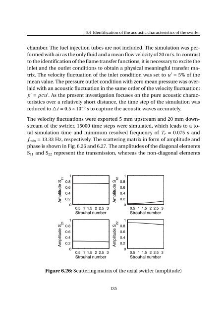The velocity fluctuations were exported 5 mm upstream <strong>and</strong> 20 mm downstream <strong>of</strong> the swirler. 15000 time steps were simulated, which leads to a total simulation time <strong>and</strong> minimum resolved frequency <strong>of</strong> T t = 0.075 s <strong>and</strong> f min = 13.33 Hz, respectively. The scattering matrix in form <strong>of</strong> amplitude <strong>and</strong> phase is shown in Fig. 6.26 <strong>and</strong> 6.27. The amplitudes <strong>of</strong> the diagonal elements S 11 <strong>and</strong> S 22 represent the transmission, whereas the non-diagonal elements Amplitude S Amplitude S 21 11 1 0.8 0.6 0.4 0.2 0 1 0.8 0.6 0.4 0.2 0 0.5 1 1.5 2 2.5 3 Strouhal number 0.5 1 1.5 2 2.5 3 Strouhal number Amplitude S Amplitude S 22 12 1 0.8 0.6 0.4 0.2 0 1 0.8 0.6 0.4 0.2 0 0.5 1 1.5 2 2.5 3 Strouhal number 0.5 1 1.5 2 2.5 3 Strouhal number Figure 6.26: Scattering matrix <strong>of</strong> the axial swirler (amplitude) 135
Page 1:
Technische Universität München In
Page 4 and 5:
und ihre Geduld besonders für die
Page 7 and 8:
Contents 1 Introduction 1 1.1 Techn
Page 9 and 10:
CONTENTS 7.2.2 Impact</stro
Page 11 and 12:
Nomenclature G stretch factor [-] h
Page 13 and 14:
Nomenclature λ air-fuel</s
Page 15 and 16:
1 Introduction 1.1 Technology backg
Page 17 and 18:
1.2 Thermo-acoustic instabilities 1
Page 19 and 20:
1.2 Thermo-acoustic instabilities d
Page 21 and 22:
1.3 Control of the
Page 23 and 24:
1.3 Control of the
Page 25 and 26:
1.4 Intention and
Page 27 and 28:
1.5 Terminology and</strong
Page 29 and 30:
1.5 Terminology and</strong
Page 31 and 32:
2 Numerical analysis of</st
Page 33 and 34:
2.1 Overview of me
Page 35 and 36:
2.1 Overview of me
Page 37 and 38:
2.1 Overview of me
Page 39 and 40:
2.2 Flame dynamics of</stro
Page 41 and 42:
Page 43 and 44:
Page 45 and 46:
Page 47 and 48:
2.3 Identification of</stro
Page 49 and 50:
Page 51 and 52:
Page 53 and 54:
Page 55 and 56:
Page 57 and 58:
3 Acoustics Before analyzing the ac
Page 59 and 60:
3.1 Basic acoustic equations as a f
Page 61 and 62:
3.2 Linear acoustic equations Here,
Page 63 and 64:
3.2 Linear acoustic equations p ′
Page 65 and 66:
3.3 Acoustic network model p ′ (x
Page 67 and 68:
3.3 Acoustic network model matrix e
Page 69 and 70:
3.3 Acoustic network model The <str
Page 71 and 72:
3.3 Acoustic network model where A
Page 73 and 74:
3.3 Acoustic network model coming c
Page 75 and 76:
3.3 Acoustic network model Z i Air
Page 77 and 78:
3.3 Acoustic network model pressure
Page 79 and 80:
3.3 Acoustic network model The eige
Page 81 and 82:
3.3 Acoustic network model tine. To
Page 83 and 84:
4 Modeling of turb
Page 85 and 86:
4.1 Theory and num
Page 87 and 88:
4.1 Theory and num
Page 89 and 90:
4.2 Theoretical and</strong
Page 91 and 92:
Page 93 and 94:
Page 95 and 96:
5 System Identification Flame trans
Page 97 and 98: 5.1 Model structures and</s
Page 99 and 100: 5.2 System Identification 5.2 Syste
Page 101 and 102: 5.3 Excitation signals the zero mea
Page 103 and 104: 5.4 A posteriori validation <strong
Page 105 and 106: 5.4 A posteriori validation <strong
Page 107 and 108: 5.5 Proof
Page 119 and 120: 6 Numerical simulation MISO model i
Page 121 and 122: 6.1 Practical premixed combustor co
Page 129 and 130: 6.2 Steady-state simulations <stron
Page 131 and 132: 6.2 Steady-state simulations <stron
Page 133 and 134: 6.3 Identifiction of</stron
Page 147: 6.3 Identifiction of</stron
Page 151 and 152: 6.4 Identification of</stro
Page 153 and 154: 7 Acoustic analysis Once the acoust
Page 155 and 156: 7.1 Setup of the a
Page 157 and 158: 7.2 Acoustic network model results
Page 181 and 182: 8 Summary and Conc
Page 183 and 184: The flame element of</stron
Page 185 and 186: Bibliography [1] Verband</s
Page 187 and 188: BIBLIOGRAPHY [18] L. Crocco. Theore
Page 189 and 190: BIBLIOGRAPHY [36] A. Giauque, L. Se
Page 191 and 192: BIBLIOGRAPHY [54] J.J. Keller, W. E
Page 193 and 194: BIBLIOGRAPHY [72] T. Lieuwen <stron
Page 195 and 196: BIBLIOGRAPHY Number 98-GT-269 in In
Page 197 and 198: BIBLIOGRAPHY [112] T. Sattelmayer.
Page 199 and 200:
BIBLIOGRAPHY [130] A. Widenhorn. pr
Page 201 and 202:
A.2 Estimation of
Page 203 and 204:
A.3 Main flow parameters an
show all

Impact of fuel supply impedance and fuel staging on gas turbine ...

You also want an ePaper? Increase the reach of your titles

Delete template?

Save as template?