2011 EMC Directory & Design Guide - Interference Technology

testing & test equipment
M e a s ur e m e n t Un c e r ta in t y f o r C o nduc t e d, R a di at e d Emi s s i o n s
United Kingdom Accreditation
Service - LAB34 - The Expression of
Uncertainty in EMC Testing - Edition
1 - August 2002.
Two Examples of Measurement
Uncertainty – Conducted
Emissions and Radiated
Emissions
The following paragraphs go into detail
on the MU for instrumentation
for conducted and radiated emissions.
The presentation of the table is different
from what is seen in the usual MU
references; namely CISPR 16-4-2 and
LAB34.
First of all, we have listed our
Sources of Uncertainty in the two
accompanying tables in order of the
largest contributor to the smallest
contributor. This allows us to see which
Source is contributing the most to the
Measurement Uncertainty.
Secondly, we are going to assume
the sensitivity coefficient is one for
all our contributing factors thus
eliminating one column in our table of
standard uncertainties (the sensitivity
coefficient is effectively a conversion
factor from one unit to another). This is
logical in the EMC Engineering world
since almost every contributing factor
is quoted in "dBs."
Our table then becomes easier
to understand with the Value of the
Sources of Uncertainty (second column)
being divided by its accompanying
Probability Distribution Function
Divisor (fourth column) to arrive at
the standard uncertainty for that
uncertainty component [U(y)] in the
fifth column. The sixth column is arrived
at by simply squaring the "result
in the fifth column." Summing all the
factors in the sixth column and taking
the square root of the total, we arrive at
the Combined Standard Uncertainty.
The Expanded Uncertainty is achieved
by multiplying the Combined Standard
Uncertainty by two for a coverage of
95%. The Expanded Uncertainty is the
engineer’s “padding factor” to make
sure he has the answer covered in the
range of values quoted.
By using the Expanded Uncertainty,
we arrive at a 95% probability that the
true answer lies within a band of values
bracketed by the measured value plus
or minus the Expanded Uncertainty.
Conducted Emissions
The above table assumes typical values
from LAB34 and CISPR 16-4-2 and is
ordered from the largest contributor
to the smallest contributor. In order
to reduce the Combined Standard Uncertainty,
the lab should start with the
largest contributors and try to reduce
their values.
In the case of the conducted emissions,
the largest contributor is the
LISN Impedance.
A check of the calibration certificate
of one of the well-known calibration
labs in the country indicates a maximum
measurement uncertainty of plus
or minus 1.2 ohms for a LISN Calibration.
This maximum uncertainty was
arrived at by the calibration lab by a
Type A evaluation using at least 10
data sets. The 1.2 ohms translates into a
value in dBs equivalent to +/- 1.6 dB. If
we substitute this 1.6 dB value into the
table for the present 2.7 dB, we lower
our combined standard uncertainty
to 1.71 dB which lowers our Expanded
Uncertainty to 3.42 dB or a reduction
of 0.32 dB. One of the reasons that the
LISN factor reduction does not make a
big difference is that it is divided by the
square root of 6 (2.449) for a triangular
distribution.
We would next have to look at the
biggest contributors to the Measurement
Uncertainty after the LISN Impedance.
They would be the Receiver
Pulse Amplitude and the Receiver
Pulse Repetition. One way to reduce
these two contributions from the Re-
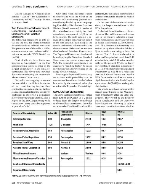
Source of Uncertainty
Value dB
Probability
Distribution
Divisor
U(y)
dB
(U(y))2
dB
Site Imperfections 4.00 Triangular 2.449 1.63 2.667
Mismatch -1.25 U-shaped 1.414 -0.88 0.781
Receiver Pulse Amplitude 1.50 Rectangular 1.732 0.87 0.750
Receiver Pulse Repetition 1.50 Rectangular 1.732 0.87 0.750
Receiver Sine Wave 1.00 Normal 2 2.000 0.50 0.250
Antenna Factor Calibration 1.00 Normal 2 2.000 0.50 0.250
Miscellaneous Factors Various Various 0.84 0.701
Measurement Distance Variation 0.60 Rectangular 1.732 0.35 0.120
Combined Standard Uncertainty √6.269 = 2.50
Expanded Uncertainty 5.00
Table 2. 30 MHz to 300 MHz with a biconical antenna in the vertical polarization – 3 & 10 meters.
32 interference technology emc Directory & design guide 2011